The Anatomy of the Least Squares Method, Part Four

Modeling GPT activations

Hey! It’s Tivadar from The Palindrome.

The legendary Mike X Cohen, PhD is back with the final part of our deep dive into the least squares method, the bread and butter of data science and machine learning.

Enjoy!

Cheers,
Tivadar

---

By the end of this post series, you will be confident about understanding, applying, and interpreting regression models (general linear models) that are solved using the famous least-squares algorithm. Here’s a breakdown of the post series:

Part 1: Theory and math. If you haven’t read this post yet, please do so!

Part 2: Explorations in simulations. You learned how to simulate and visualize data and regression results.

Part 3: real-data examples. Here you learned how to import, inspect, clean, and analyze a real-world dataset using the statsmodels, pandas, and seaborn libraries.

Part 4 (this post): modeling GPT activations. We’ll dissect OpenAI’s LLM GPT2, the precursor to its state-of-the-art ChatGPT. You’ll learn more about least-squares and also about LLM mechanisms.

Following along with code

Seeing math come alive in code gives you a deeper understanding and intuition — and that warm fuzzy feeling of confidence in your newly harnessed coding and machine-learning skills. You can learn a lot of math with a bit of code.

Here is the link to the online code on my GitHub for this post. I recommend following along with the code as you read this post.

---

📌 The Palindrome breaks down advanced math and machine learning concepts with visuals that make everything click.

Join the premium tier to get access to the upcoming live courses on Neural Networks from Scratch and Mathematics of Machine Learning.

---

Import and inspect the GPT2 model

A large language model (LLM) is a deep-learning model that is trained to input text and generate predictions about what text should come next. It’s a form of generative AI because it uses context and learned worldview information to generate new text.

If you think LLMs are so complicated that they are impossible to understand, then I have bad news for you… you’re wrong! LLMs are not so complicated, and you can learn all about them with just a high-school-level math background. If you’d like to use Python to learn how LLMs are designed and how they work, you can check out my 6-part series on using machine-learning to understand LLM mechanisms here on Substack.

There are two goals of this post: (1) to show you how easy it is to import and inspect an LLM, and (2) to apply the least-squares algorithm to model some internal activations while an LLM processes text.

Let’s begin with that first goal.

The code block below imports OpenAI’s GPT2 model using a library developed by a company called HuggingFace (cute name for an AI company, don’t you think?).

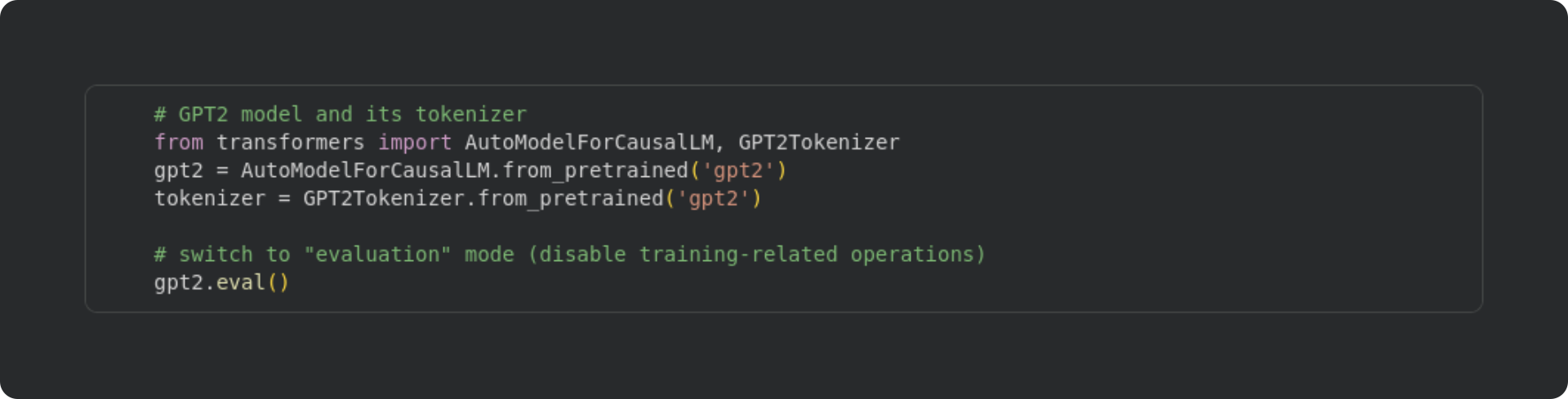
GPT2 is the precursor to OpenAI’s ChatGPT models. The architecture and algorithms are the same, but GPT2 is smaller. It’s used very often for learning about and studying LLMs, analogous to how the MNIST dataset of hand-written digits is used for learning about computer vision.

Anyway, that code block imports the model (variable gpt2) and a “tokenizer.” I’ll explain what a tokenizer is in the next section; first I want to show the overview of the GPT2 architecture.

GPT2LMHeadModel(
  (transformer): GPT2Model(
    (wte): Embedding(50257, 768)
    (wpe): Embedding(1024, 768)
    (drop): Dropout(p=0.1, inplace=False)
    (h): ModuleList(
      (0-11): 12 x GPT2Block(
        (ln_1): LayerNorm((768,), eps=1e-05, elementwise_affine=True)
        (attn): GPT2Attention(
          (c_attn): Conv1D(nf=2304, nx=768)
          (c_proj): Conv1D(nf=768, nx=768)
          (attn_dropout): Dropout(p=0.1, inplace=False)
          (resid_dropout): Dropout(p=0.1, inplace=False)
        )
        (ln_2): LayerNorm((768,), eps=1e-05, elementwise_affine=True)
        (mlp): GPT2MLP(
          (c_fc): Conv1D(nf=3072, nx=768)
          (c_proj): Conv1D(nf=768, nx=3072)
          (act): NewGELUActivation()
          (dropout): Dropout(p=0.1, inplace=False)
        )
      )
    )
    (ln_f): LayerNorm((768,), eps=1e-05, elementwise_affine=True)
  )
  (lm_head): Linear(in_features=768, out_features=50257, bias=False)
)

If this is your first encounter with LLMs in Python, then that overview probably looks intimidating. At a quick glance: each tab-indented section describes a different part of the model and provides some information about the sizes of the parameter matrices. The (h) is for the hidden layers, which comprise 12 transformer blocks. A transformer is the heart and soul of a language model, and is made of two parts: attention ((attn)) and MLP.

The attention subblock is perhaps the most famous part of a language model, and that will be our main focus here in this post. Briefly, the attention subblock analyzes the text you’ve given to the model (e.g., the prompt you write to ChatGPT or the text in the pdf you upload) and find pairs of words that are important. For example, in the first sentence of this paragraph, the word pair [“subblock”, “focus”] is relevant for generating new text, but the word pair [“the”, ”of”] is not relevant. The attention subblock calculates adjustments that modify how each word is represented, according to the importance of those word-pairs. In the regression analysis here, we will focus on those adjustments.

But before setting up the model, you need to know how to transform text into tokens and then how to access the internal model activations.

Tokenize text and get attention adjustments

You interact with chatbots like ChatGPT or Claude using text, but LLMs don’t actually read text. Instead, they read a sequence of integers that correspond to words and subwords. Those are called tokens. For example, the word “ rock” is token 3881.

GPT2 models have a vocabulary of 50,257 tokens. Many of those tokens correspond to whole words, others are digits, punctuations, subwords (e.g., “om”), and bits of code (e.g., “<\html”).

The goal of this section is to start with human-readable text, transform it into tokens, and then extract the attention adjustment vectors from the LLM. We’ll use those data for the statistical modeling in the next section.

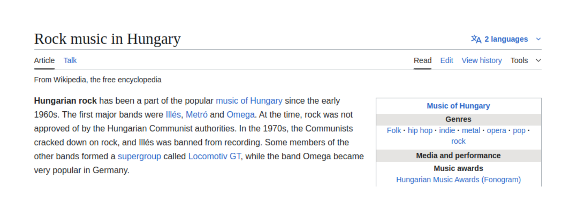
The text I’ve chosen to work with in this post is a paragraph about Hungarian rock music from Wikipedia:

Here’s a screenshot of what the code looks like (some of the code lines are longer than the screenshot, but you can see the entire code file on my GitHub):

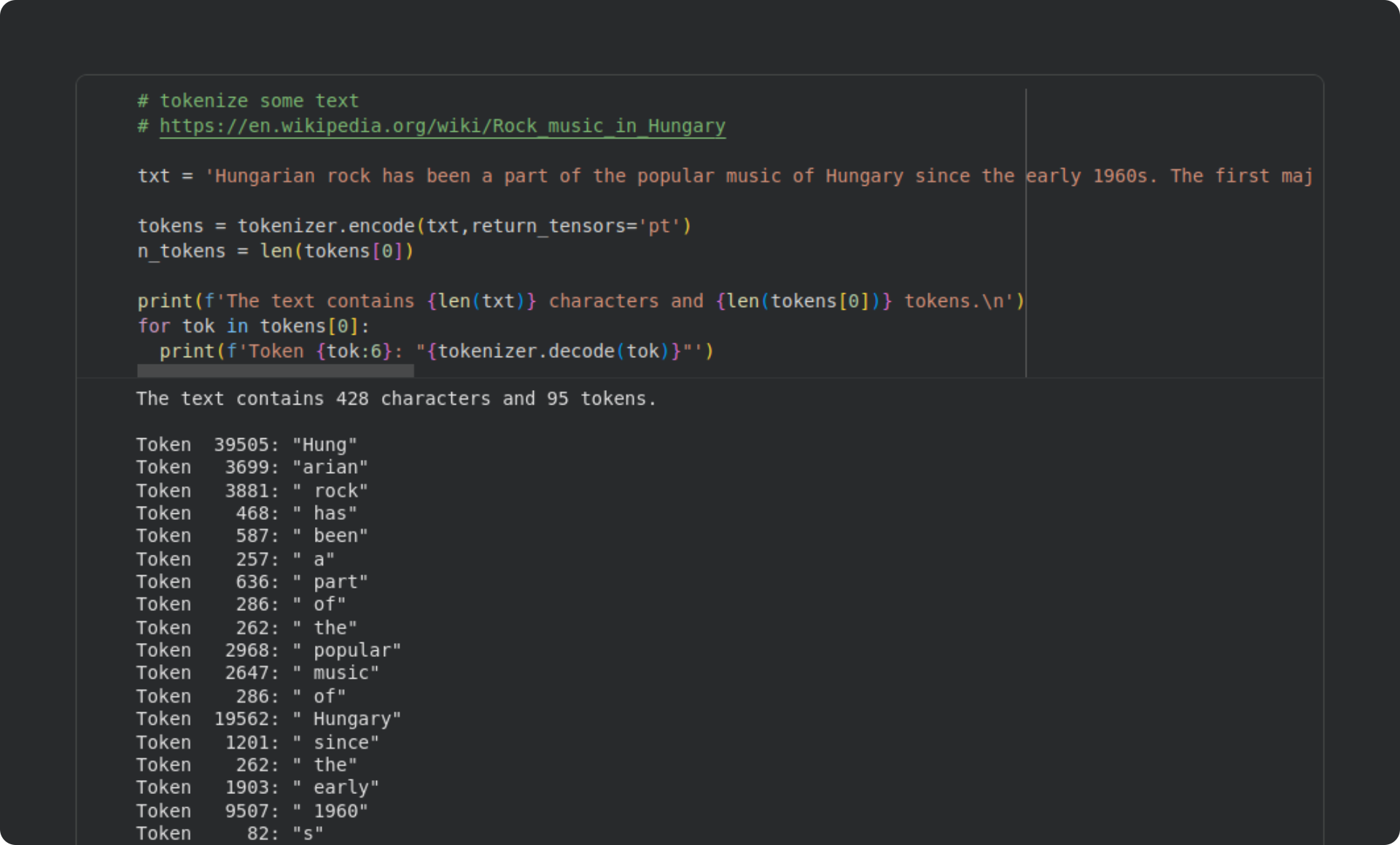
That paragraph contains 428 characters but only 95 tokens. That’s almost an 80% compression of the text. Tokenization compresses language (in many but not all languages), which helps improve LLMs’ memory efficiency.

At the bottom of that code block, I printed out the token indices and their corresponding text tokens. Many common words map onto one token, while other words get split into multiple tokens (e.g., “Hungarian” is coded as “Hung” + “arian”). GPT models often have spaces before whole words. That’s a result of how the tokenization algorithm (called the byte-pair-encoding algorithm) segments written language based on statistical co-occurrences; for example, “th” gets chunked into one token whereas “tq” is two tokens.

Anyway, we now have 95 tokens that we can input into the model. Providing input to a language model is called a “forward pass” and is what happens when you type a prompt into ChatGPT and press the Enter key.

The goal of the regression analysis in the next section will be to predict the attention adjustment to the current token based on the attention adjustments to the previous two tokens. In other words, if the model made a large adjustment to the previous tokens, does it also make a large adjustment to the current token?

To run that analysis, we need to access the internal calculations inside the attention subblock. Those are not readily available from outside the model, but PyTorch models have a special method, called a hook function, that allows us to access the hidden internals of models. A hook function is a regular python function that gets evaluated when a specified layer in the model is run. The code block below shows how I created a hook function that I implanted into each layer (“layer” referring to a transformer block that contains an attention subblock). I will explain each numbered part of the code below.

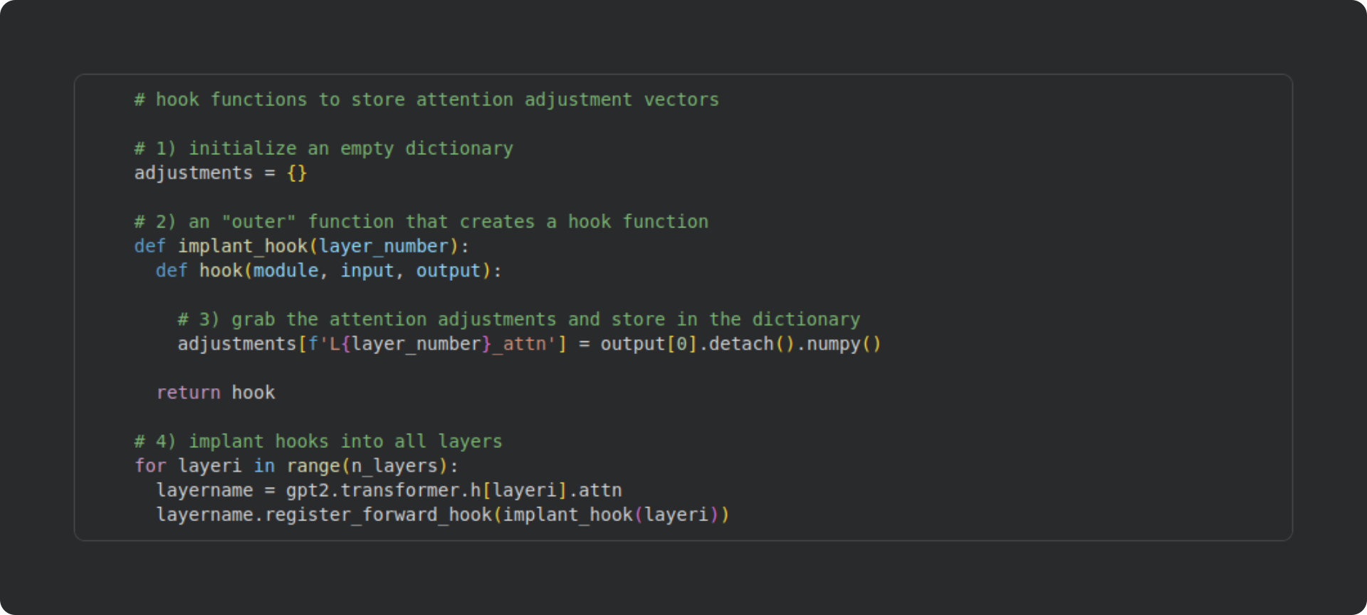
1. Initialize an empty dictionary in the global Python scope (accessible anywhere to any function). The hook function will populate this dictionary with the outputs of the attention calculations.

2. Here you see two embedded functions. The “outer” function (implant_hook) is actually just a wrapper to pass an input argument (layer_number) into the hook function. The hook function is what gets implanted into the model at a key location during the forward pass (I’ll explain that in #4).

3. Hook functions can be as simple or as complicated as you need them to be. They’re just normal Python functions. For this demo, the hook function is very simple — I just grab a copy of the output of the attention subblock, change the data type from PyTorch tensor to NumPy array, and then store it in the activations dictionary in a key named for the layer from which the activations are extracted.

4. Here’s where the hooks are implanted. I loop over all the layers (all the transformer blocks), and use the built-in PyTorch method register_forward_hook to install the hook function.

With those hook functions implanted, we can now run a forward pass of the model. When we input the tokens, the model will run its calculations to generate predictions about next tokens, and in so doing, it will run through the attention algorithm and copy the adjustments into the dictionary.

The code block below shows the forward pass and some information about the adjustments that were stored in the dictionary.

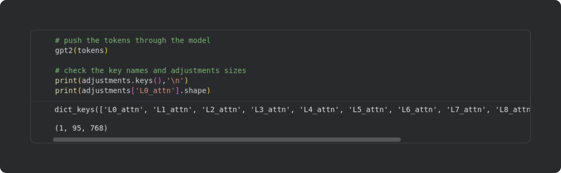
There are several outputs that you can get from the model (e.g., out=gpt2()). However, for this demo, we don’t want the model outputs; we want the model internals. Those were copied into the adjustments dictionary, and you can see the list of keys that were created by the hook functions. The final line of code prints the shape of the NumPy array from one of the attention blocks. It is of size 1 × 95 × 768. “1” corresponds to the number of text sequences that we inputted (it is possible to batch multiple sequences to be processed in parallel); “95” is the number of tokens in the sequence, and “768” is the embeddings dimensionality. Embeddings are a dense representation of the tokens, and allow the language model to modify the tokens according to context and world knowledge. The attention algorithm calculates adjustments to those embeddings vectors, and our hook functions copied those adjustments into the dictionary so we can analyze them.

Those 768-dimensional embeddings adjustments provide rich, detailed, and complex information. For our purposes here, though, we will summarize the embeddings adjustments by measuring their magnitude.

The magnitude of the adjustment vector is its norm. If you’re familiar with linear algebra, then you’ll remember that the vector norm is the square root of the sum of the squared elements of a vector. For example, the norm of the vector [1,0,-3] is sqrt(1+0+9) = sqrt(10) = 3.16. The smaller the norm, the smaller the adjustment to the embeddings vector.

We will use those adjustment vector norms in the regression analysis, but before we start building statistical models, it’s a good idea to inspect the data through visualizations.

In the code block below, I extract the norm of the vectors, plot them, and make a histogram. Please try to understand what the code does before reading my explanations below. I’ll show the plots below that.

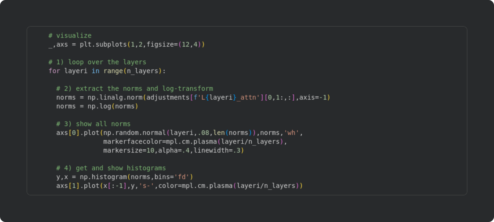
1. Loop over all 12 layers (transformer blocks).

2. Calculate the norms of the attention adjustment vectors for all of the tokens except the first one. The first token in a sequence is usually an outlier because the model has no previous context to generate next-token predictions, and is therefore excluded. The norms are all positive (by definition) and long-tailed, and so taking the logarithm of the norms helps make them more suitable for a regression analysis — same as in the previous post with the apartment sales dataset.

3. Here I make a scatter plot of the activation norms. The random.normal input creates tiny x-axis jitters that help visualize the density of the data.

4. To examine the distribution of attention norms, I extract histograms. There’s only 94 tokens, so rather than specifying the number of bins, I use the Freedman-Diaconis guideline to algorithmically select an appropriate number of histogram bins.

The figure below shows the result of running that code.

Figure 1. The left panel shows a scatter plot of the attention adjustment vector norms (log scaled; each dot corresponds to one token in the prompt text). The right panel shows histograms of the adjustment norms for each layer, with the color of the lines corresponding to the layer number as in the left panel.

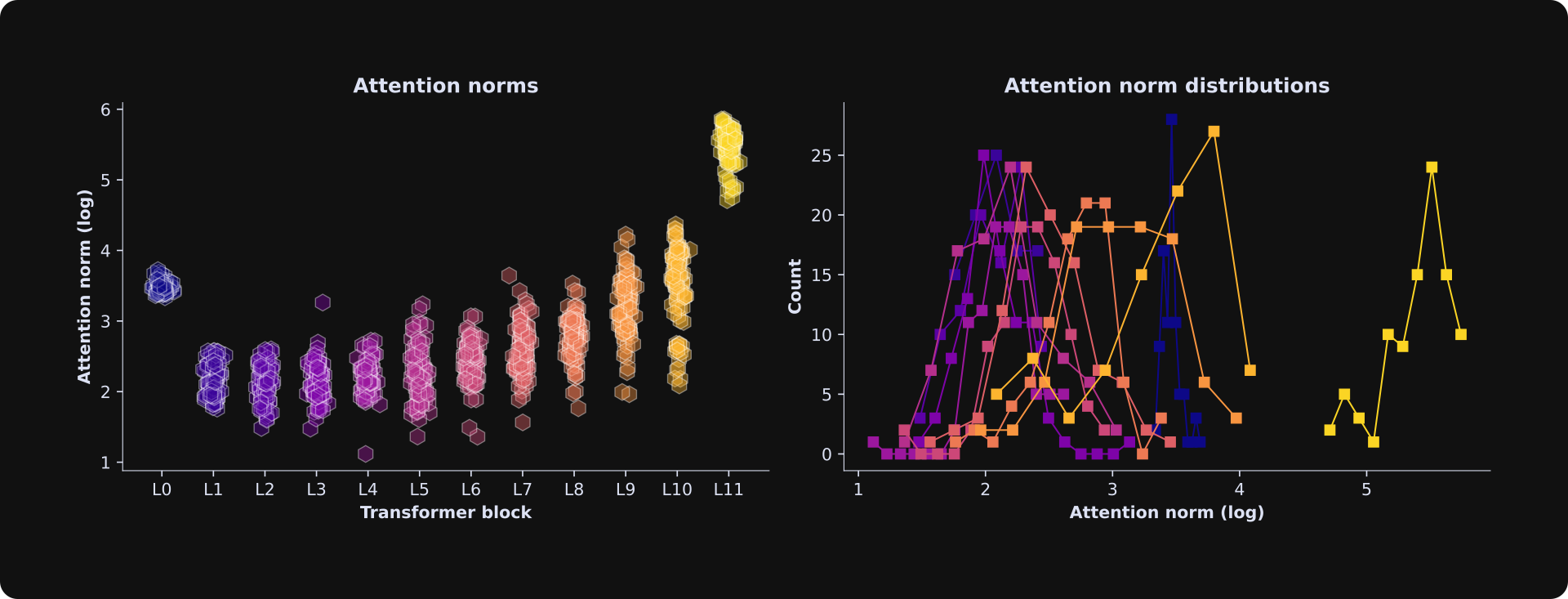
The first layer has relatively large adjustments that are all clustered together. Here’s why: The initial embeddings reflect the words themselves and not their context, and L0 is the first opportunity for the model to adjust the vectors according to the specific context of the prompt text. For example, the word “bark” has one embeddings vector before L0, regardless of whether the text is about a dog or a tree; at L0, the model can begin adjusting the embeddings vector depending on the local context.

Thereafter, as the text moves deeper into the model (later transformer blocks), the embeddings vectors shift from pointing towards the word in the input prompt, to predictions about what tokens should come next (the LLM’s generative output text). That requires additional adjustments.

The right panel in that figure shows histograms of the norms. These are all fairly normal — not perfectly Gaussian, but each layer has one central peak with decaying counts on either side. That’s a suitable distribution for a least-squares regression analysis.

I’m sure you are super excited to start the statistical modeling! Keep reading 😁

Build and fit a model for one transformer

The goal of our analysis is to determine whether the attention adjustment to the current token can be predicted from the attention adjustment to the two preceding tokens.

Translated into an equation, the regression model we’ll test here is the following:

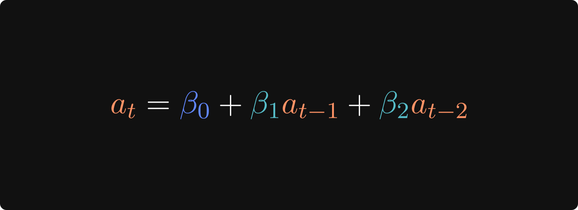
Where a_t is the magnitude of the attention adjustment on token t, 𝛽₀ is the intercept, and 𝛽₁ and 𝛽₁ are the impacts of the adjustments on the previous tokens.

The code block below shows how I created a design matrix for one layer in the language model. I will extend this to all the layers in the next section; for now, just focus on how the design matrix and dependent variables are created. As always, please try to understand the code before reading my explanations below.

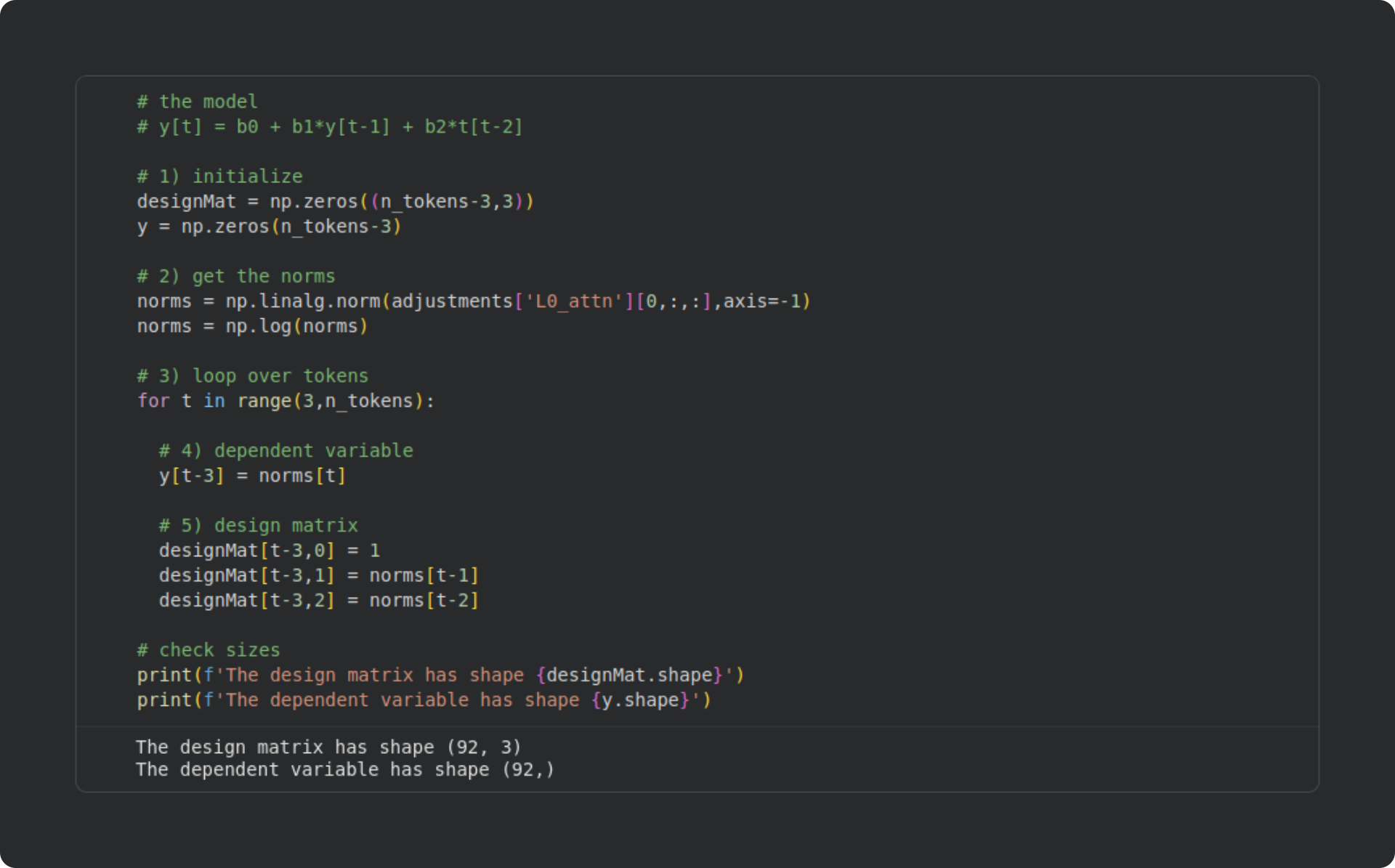
1. Here I initialize NumPy arrays for the design matrix and dependent variable. Those arrays are n_tokens - 3 because (1) I ignore the first token in the sequence and (2) the model will attempt to predict the current norm based on the two preceding norms. For these reasons, the first usable prediction is the fourth data point (index 3).

2. Calculate the log-transformed norms of the attention adjustments, as I showed earlier.

3. Here’s where I build the design matrix. I start the for-loop at index 3, then set the dependent variable (y) to be the current-token norm, and I define the corresponding row in the design matrix to be an intercept term (“1”) and the norms from the previous two tokens.

Now that we have a design matrix and a dependent variable, we can fit a least-squares model using sm.OLS — exactly how I described in the previous post. Here’s the code and the summary output:

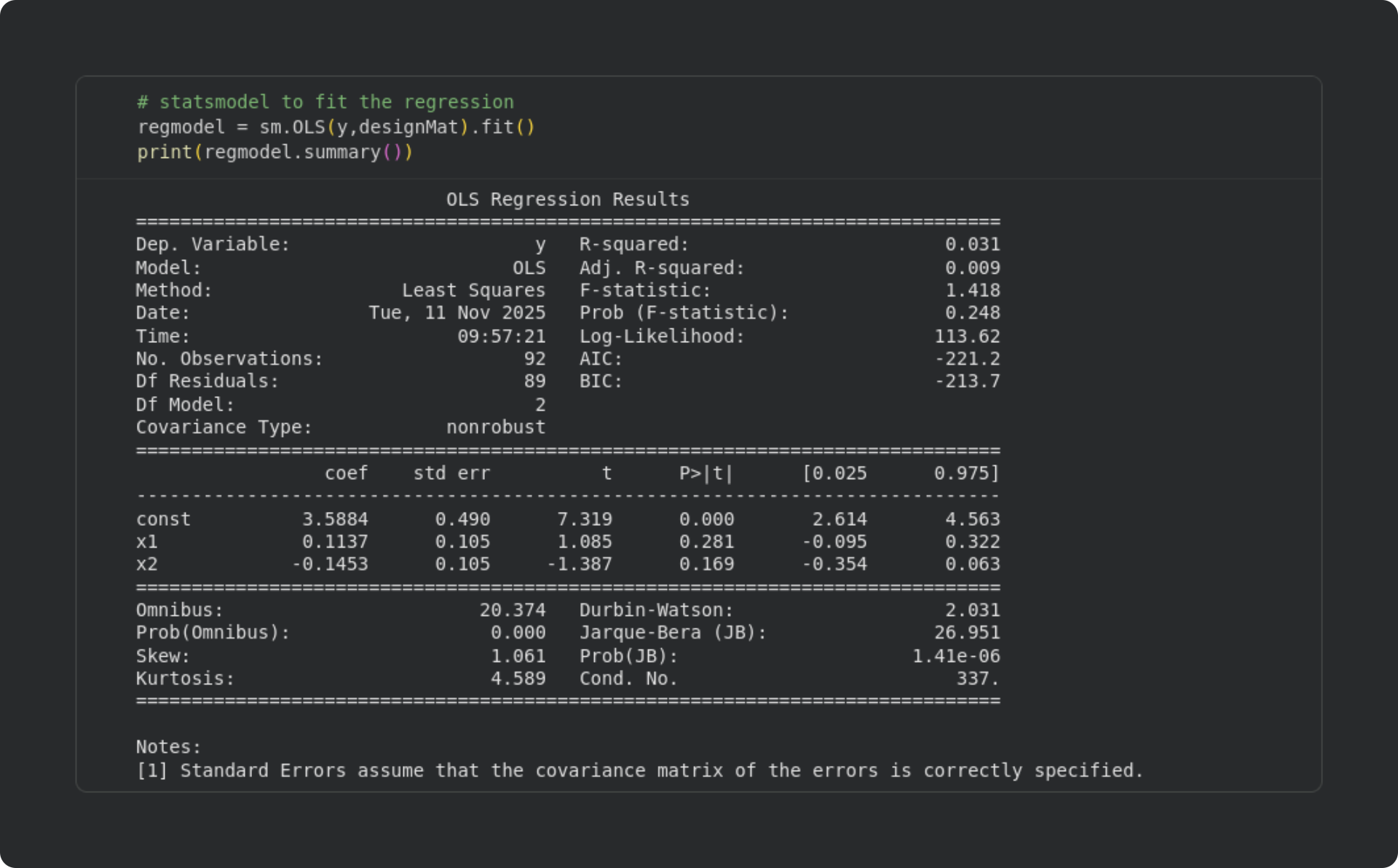
Looking through this summary table, we can see that the R² is fairly low, and the two previous-token betas are non-significant. The intercept (const) is significant, but remember from the previous post that that’s not so interesting because it just means that the average log-norm is greater than zero.

That analysis was just for the first transformer block. The next goal is to take the code and wrap it inside another for-loop over all the transformer layers.

But before looping over all the layers, there’re two more quick demos I want to show.

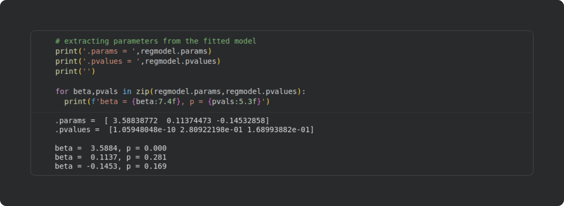
First is how to extract the numbers from that summary table. That simply involves calling the attributes of the model object. The two attributes we’ll use here are the beta values (.params) and the p-values (.pvalues).

Second is a confirmation that the least squares analysis I taught you in earlier posts gives the same results as sm.OLS. For that, we can repeat the least-squares analysis using NumPy.

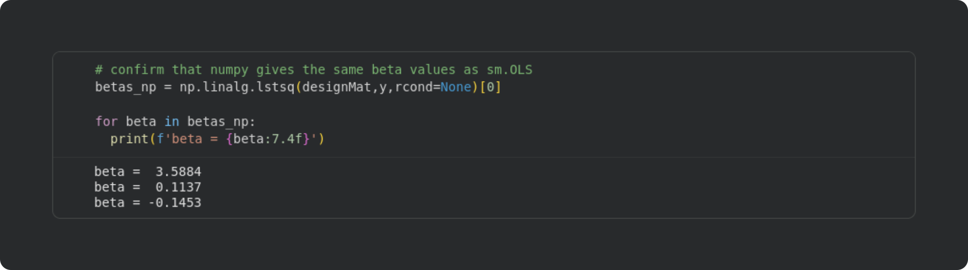
The betas from NumPy match the ones from statsmodels.

Whether to calculate least-squares directly in NumPy or use the statsmodels library depends on your goals: If you only need the beta values, then it’s easier and simpler to stick with NumPy. But on the other hand, getting the detailed information like p-values to evaluate statistical significance would be much more work with NumPy but is straightforward with statsmodels.

Run the regression for all layers

The code block below extracts the attention adjustment norms, creates a design matrix, fits the model, and extracts the beta and p-values. My explanations below.

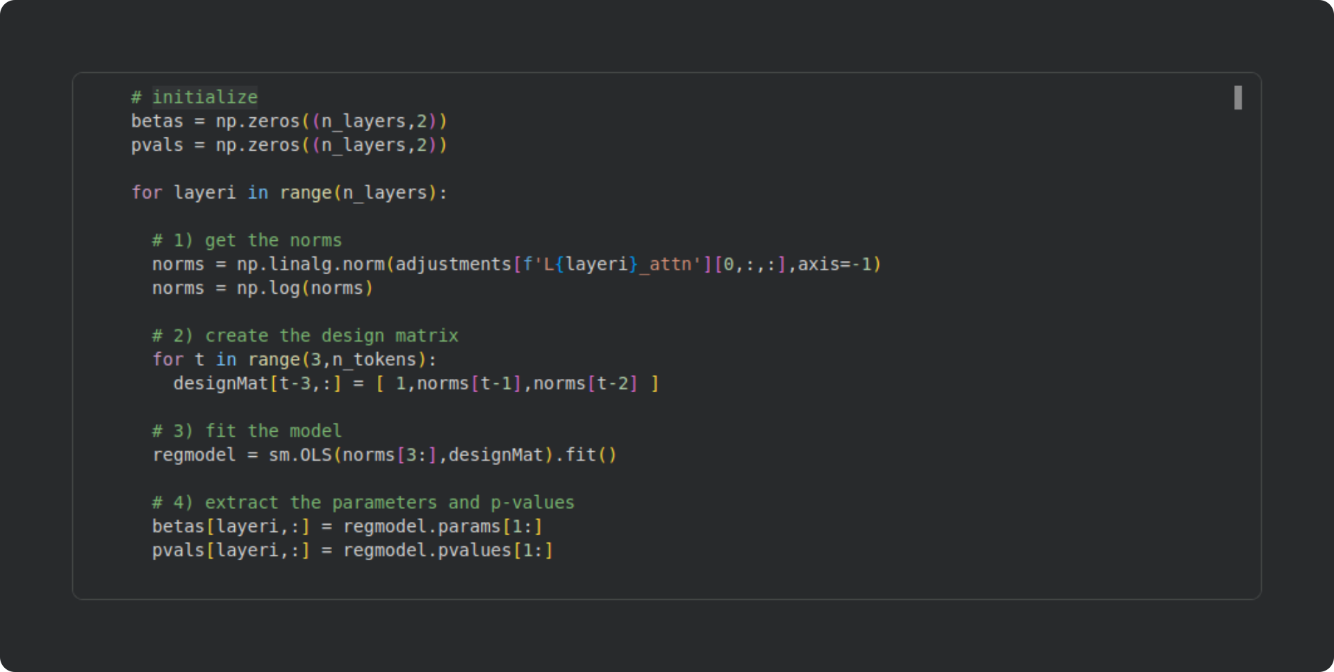
1. Extract the norms of the attention adjustments and log-transform. It’s the same code as in the previous section, but the layer number for the key name in the dictionary is soft-coded.

2. Here I use multiple assignment to create the design matrix in one line instead of three. If you’d like a little coding challenge, you can create the design matrix with no for-loops! (Hint: concatenate)

3. Here I fit the model as in the previous section. Rather than creating a separate Python variable for the model’s dependent variable, I directly input the norms array.

4. Extract the beta values and corresponding p-values from the model, indexing [1:] because the first parameter is the intercept. You can extend the code by extracting additional model statistics, for example the adjusted R². So many possibilities for additional explorations 🙂

The final results are visualized in the figure below. The x-axis shows the transformer block, the y-axis shows the beta coefficients for the two predictor variables, and the markers are solid if the beta is statistically significant (p < .05) or a white “x” if the beta is non-significant (p > .05).

Figure 2. Beta coefficients (y-axis) over the transformer blocks (x-axis) showing the impact of preceding attention adjustment norms on the current adjustment norms. Full markers indicate statistically significant betas; “x” markers indicate non-significant markers. A positive beta indicates that when the previous token has a large adjustment, the current token also has a large adjustment.

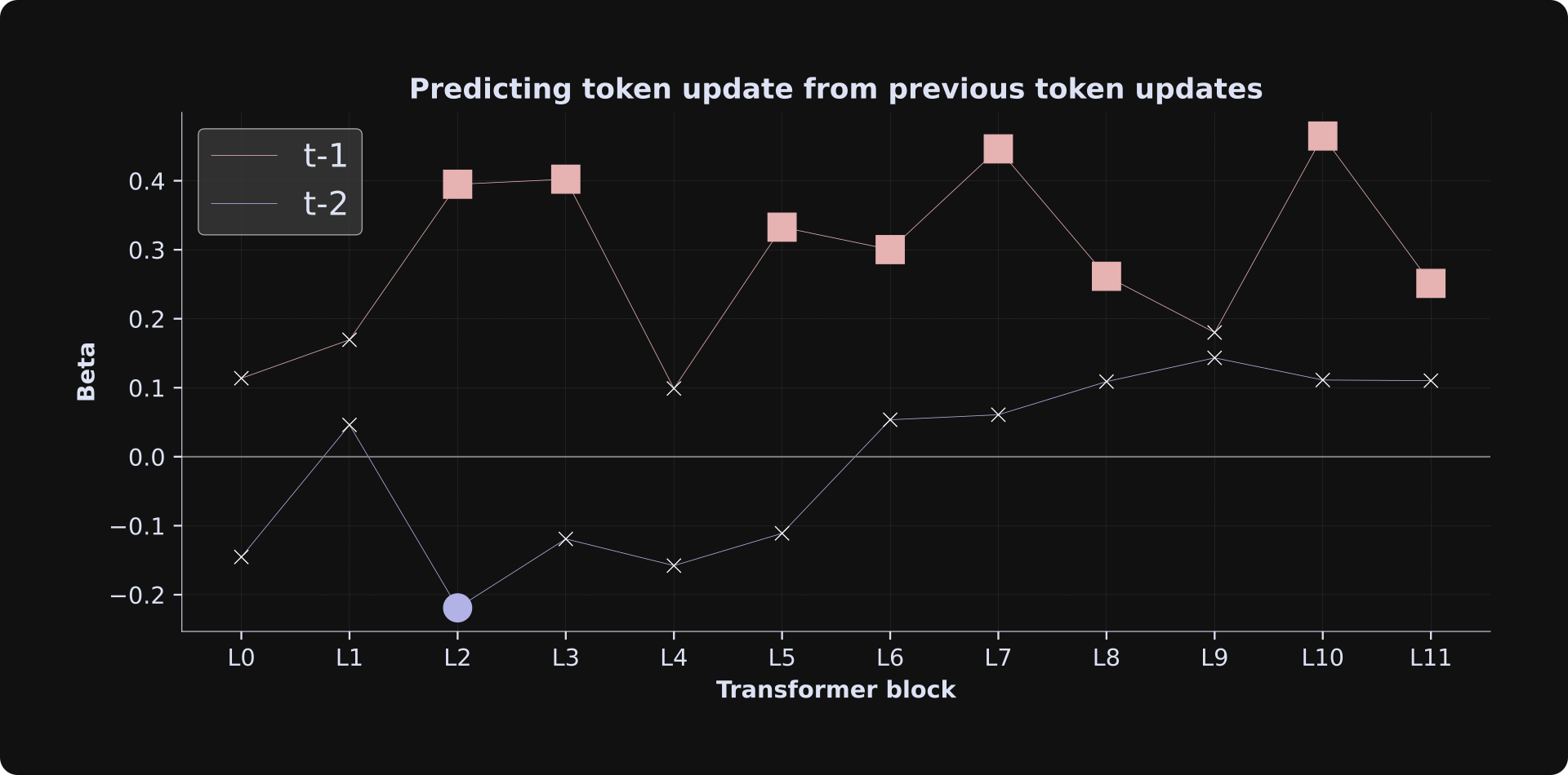
The results indicate that the previous token’s adjustment predicts the current token’s update magnitude, but not the adjustment from two tokens previously. Numerically, the t-2 adjustment negatively predicts the current token update (that is, when the t-2 token adjustment was larger, the current token update was smaller) in earlier layers, although most of the betas are non-significant, so you should interpret that result cautiously.

Further words of caution: This analysis was done with a small amount of text taken from one Wikipedia article. In real LLM research, you would use a much larger amount of data taken from a variety of sources. You would also extend this research to determine the nature and importance of the adjustments, and possibly run separate analyses according to part of speech (e.g., nouns, verbs, adjectives) or other linguistically insightful characteristics. It would also be a good idea to supplement this research with causal interventions, where you could manipulate the nature and size of the adjustments to determine the impact on downstream processing and next-token prediction. All that said, these are comments about a full scientific investigation; the application of least-squares and regression is the same in this little demo as it would be for a publishable scientific research program.

Also: LLM researchers are often concerned with universality, which is the question of whether the same computational principles emerge in all LLMs, or whether findings are unique to one particular model. Out of curiosity, I ran the code again using the “XL” version of the model (you can do this simply by importing ‘gpt2-xl’ instead of ‘gpt2’). The pattern of results was replicated in the larger model, which you can see below.

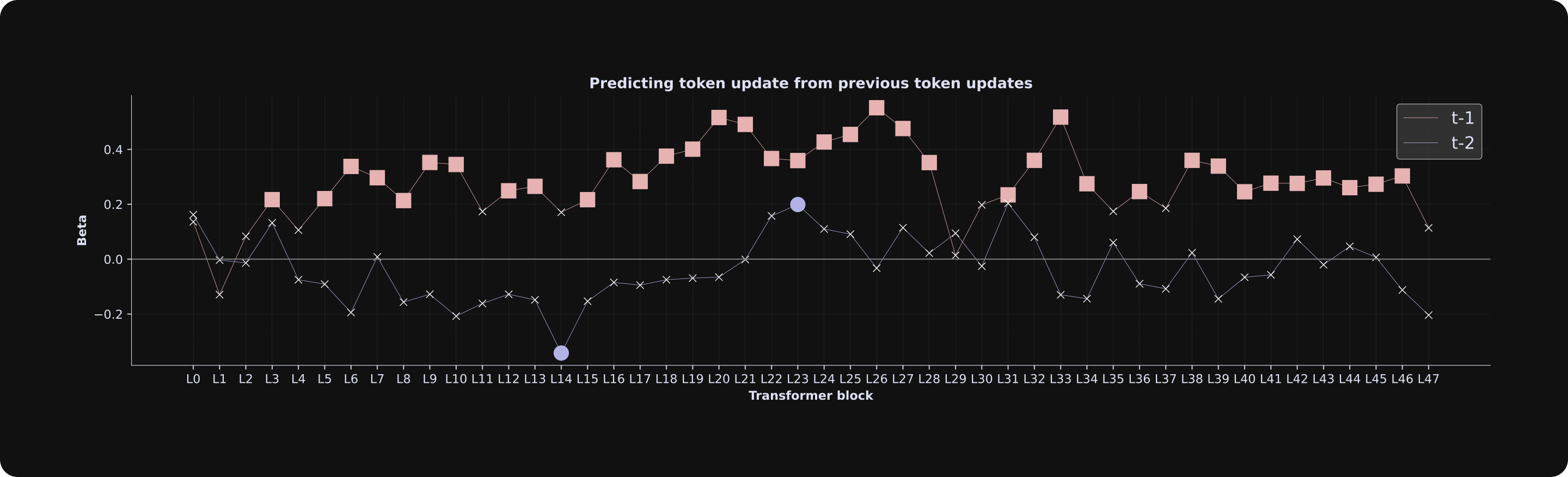
Figure 3. Same analysis and graph as shown in the previous figure, but using the “XL” version of GPT2. The architecture is the same, but the XL version is both wider and deeper, for example 48 transformer blocks instead of 12.To produce Figure 3, you re-run the code file but importing ‘gpt2-xl’ instead of ‘gpt2’ at the top of the script. You can also try running other GPT2 variants including “medium” and “large.”

Celebrate your achievements!

You’ve just completed the four-post series on least-squares.

Pat yourself on the back, eat an ice cream, go for a walk in nature, kiss your dog… do something that makes you happy and be proud of investing in your brain and in your future by learning something difficult.

… and then join me to learn more difficult topics 🤣

If you want to learn more from me (Mike X Cohen, ex-neuroscience professor and current independent educator), please subscribe to my Substack, check out my online courses (discount coupon codes are embedded in the links on my website), and read my books.

And a big shout-out to Tivadar for hosting these guest posts on his newsletter The Palindrome 🥳