
The Anatomy of the Least Squares Method, Part One
Theory and Math


Hi there! It’s Tivadar from The Palindrome.
Today’s post is the first in a series by the legendary Mike X Cohen, PhD, educator extraordinaire.
In case you haven’t encountered him yet, Mike is an extremely prolific author; his textbooks and online courses range from time series analysis through statistics to linear algebra, all with a focus on practical implementations as well.
He also recently started on Substack, and if you enjoy The Palindrome, you’ll enjoy his publication too. So, make sure to subscribe!
The following series explores the least squares method, a foundational tool in mathematics, data science, and machine learning.
Have fun!
Cheers,
Tivadar
By the end of this post series, you will be confident about understanding, applying, and interpreting the least-squares algorithm for fitting machine learning models to data. “Least-squares” is one of the most important techniques in machine learning and statistics. It is fast, one-shot (non-iterative), easy to interpret, and mathematically optimal. Here’s a breakdown of what you’ll learn:
Post 1 (what you’re reading now 🙂): Theory and math. You’ll learn what “least-squares” means, why it works, and how to find the optimal solution. There’s some linear algebra and calculus in this post, but I’ll explain the main take-home points in case you’re not so familiar with the math bits.
Post 2: Explorations in simulations. You’ll learn how to simulate data to supercharge your intuition for least-squares, and how to visualize the results. You’ll also learn about residuals and overfitting.
Post 3: real-data examples. There’s no real substitute for real data. And that’s what you’ll experience in this post. I’ll also teach you how to use the Python statsmodels library.
Post 4: modeling GPT activations. This post will be fun and fascinating. We’ll dissect OpenAI’s LLM GPT2, the precursor to its state-of-the-art ChatGPT. You’ll learn more about least-squares and also about LLM mechanisms.
Following along with code
I’m a huge fan of learning math through coding. You can learn a lot of math with a bit of code.
That’s why I have Python notebook files that accompany my posts. The essential code bits are pasted directly into this post, but the complete code files, including all the code for visualization and additional explorations, are here on my GitHub.
If you’re more interested in the theory/concepts, then it’s completely fine to ignore the code and just read the post. But if you want a deeper level of understanding and intuition — and the tools to continue exploring and applying the analyses to your own projects — then I strongly encourage following along with the code while reading this post.
Here’s a video where I explain how to get my code from GitHub and follow along using Google Colab. It’s free (you need a Google account, but who doesn’t have one??) and runs in your browser, so you don’t need to install anything.
What is least-squares and why is it important?
“Least-squares” is a solution to a problem. The problem is how to fit a mathematical model to data that balances (1) accurately capturing the data while (2) being as simple as possible.
Well, I over-stated that a bit. Most of the hard work in finding that balance is up to the human data scientist. Least-squares takes care of the math once the human has done the creative work.
Least-squares helps you in a situation like this: You have two or more variables in a dataset, and you want to predict one variable based on the other variables. Here are three examples:
The variable to predict is daily sales, and the predictor variable is the daily ad budget. You need a machine-learning model that can predict the sales revenue based on advertising expenses.
You work for a bike-share company, and want to predict the number of bike rentals per day based on the outdoor temperature, hours of daily sunshine, and day of the year.
You’re a researcher for a health study on weight loss. The variable to predict is weight lost after two months, and the predictor variables are average daily caloric intake, number of exercise minutes per week, and average daily time spent on social media.
For the two-variable case, the data can be plotted as a scatter plot as in the figure below. The least-squares algorithm gives us several pieces of information that I’ll explain below.
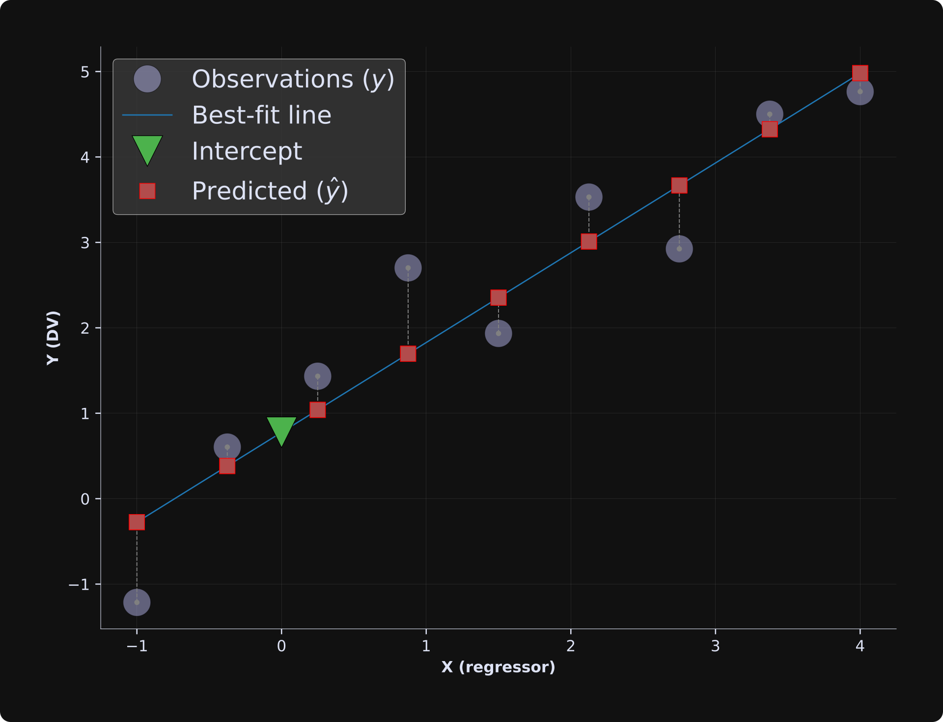
Here’s what least-squares gives us:
The best-fit line (blue line). That’s a straight line that describes the relationship between the variables. The neat thing about having a best-fit line is making predictions about data you didn’t measure. For example, we can predict that y = 3.05 when x = 2, even though we have no actual measurements at x = 2.
The predicted data (red squares). The predicted data are constrained to be on the best-fit line, and represent the value of the predictions if the model would fit the data perfectly.
Residuals (vertical dashed lines). Those are the discrepancies, or the errors, between the model predictions and the observed data. The least-squares algorithm finds the best-fit line that minimizes those error magnitudes.
Intercept (green triangle). This is the predicted observation when all predictors are set to zero. You can think of it like a “baseline” value that the model predicts, even if we have no actual baseline data.
The least-squares algorithm is all over the place in applied math: Where there’s data, there’s likely to be least-squares. To be sure, it’s not perfect, and it’s not ubiquitous. Least-squares doesn’t power LLMs, for example. Least-squares is for linear solutions, like regressions and general linear models. Well, to clarify: least-squares can identify nonlinear relationships in data, for example, polynomial regressions, as long as the model parameters are linear (meaning addition and multiplication).
Anyway, let’s make this more concrete before I explain the math.
Example: Hungarian punk makes you happy
Note: The data in this example are fake! I made up the numbers, but the conclusions might be valid. YMMV.
Let’s imagine we take a scientific research trip to Budapest and ask five randomly selected people two questions: (1) What is your overall life happiness (from 1-10) and (2) How many Hungarian punk band concerts have you been to in the past year?
We visualize the data in a scatter plot and discover something amazing:
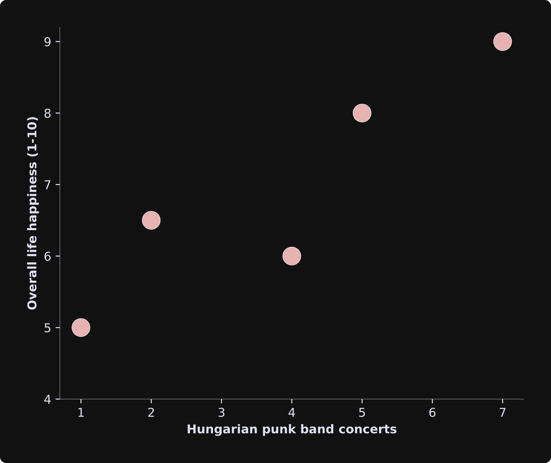
Clearly, our very serious and very scientific research has concluded that in order to live a happy and fulfilling life, you need to go to Hungarian punk rock shows.
(Note about causality: The terminology is that life happiness “depends on” punk shows, which is a variable that we can “independently” manipulate or observe. That phrasing implies a causal relationship. However, statistical models alone cannot prove causality. It’s also possible that happier people just find Hungarian punk more sonorous. Causal relationships can only be established with well-controlled experiments.)
Now our goal is to develop a statistical model that quantifies the relationship in the data. Our model needs to incorporate three variables:
Life happiness: This is the dependent variable (abbreviated to DV) — the variable we want to predict from the other variables.
Hungarian punk band concerts: This is the independent variable (abbreviated to IV) — the variable we observe (or manipulate in an experiment).
Intercept: The intercept term (also called the constant) is the expected level of life happiness for people who have been to zero punk shows.
Let’s write down some equations. The equations below are mathematical descriptions of the data shown in the figure above. The DV is blue, the IV is yellow, and the intercept is green. The beta values (𝛽) are the unknown parameters that describe the relationship between punk shows and life happiness (the punk-regressor term is orange). The goal of least-squares is to find those values.

Take a moment to see how these equations map onto each data point in the scatter plot I showed earlier.
The goal now is to solve for the two beta terms that describe the best-fitting line through the data points. Consider that when 𝛽1 is positive, it means that more punk shows are associated with higher happiness; when 𝛽1 is negative, it means that more punk shows are associated with lower happiness; and when 𝛽1 is zero, it means there is no relationship between the variables.
The equations reveal an important assumption in least-squares: the two beta parameters are the same for every person. That means we consider individual differences and other sources of variability to be “noise.” That’s an important assumption in least-squares modeling, and I’ll have more to say about that in a later post.
From a collection of equations to one matrix equation
A long list of equations is tedious, ugly, and difficult to work with. So instead, we rearrange those equations into matrices and vectors. Punk show concerts and the intercept are the two IVs, so we put those into a matrix with two columns, which is called the “design matrix.” The 𝛽s and the DV go into vectors, and we form a matrix equation:

The first column in the left matrix (the 1’s) contains the intercept terms. Those were left implicit in the collection of individual equations I showed earlier.
Now we can represent those equations compactly using matrix notation: X𝜷=y.
In the parlance of statistics, X is called the “design matrix,” 𝜷 is called the regressors or beta coefficients, and y is called the dependent variables or observations.
Least-squares solution (linear algebra)
Now, to solve the equation to find the unknown 𝜷 terms. Warning: If you’re a linear algebra noob, the equations in this section might look intimidating, and you might not understand them completely. That’s perfectly understandable; try to focus on the gist without worrying about the details.
You may be thinking that to solve for 𝜷, we simply divide by X. Indeed, if these variables reflected individual numbers and not matrices, then the solution would be simple: 𝜷 = y/X. However, division is not a defined operation in linear algebra, so we need another technique. If X were a square matrix, we could use the matrix inverse to obtain 𝜷 = X-1y. But X is almost never square — a square design matrix would mean having the same number of observations as predictors, which is a ridiculous constraint. Instead, the design matrix has more rows (observations) than columns (regressors or features). A matrix with more rows than columns is called a tall matrix and does not have a full inverse. However, it has a left-inverse, which allows us to cancel the X from the left-hand side of the equation, thereby isolating 𝜷.

I know, it’s a lot of X’s floating around, but the solution is elegant, deterministic (a.k.a., one-shot, meaning we don’t need to iterate to get an approximate solution that could change each time we re-run the code), and easy for computers to calculate with high accuracy (although there are some nuances for very large matrices, but those are solved by clever numerical algorithms).
That final equation is called the least-squares solution, and it is one of the most important sequences of matrices in all of applied mathematics. In fact, the more you study statistics, machine learning, optimization, engineering, physics, finance, or computational biology, the more you will see that equation embedded into proofs, analyses, and algorithms.
Let’s see how this looks in Python code.

What do those two beta values mean? The first number (4.58) is the intercept. That’s the level of happiness we expect in someone who has been to zero Hungarian punk shows (Tivadar cringes at the thought of someone missing out on the joy of Hungarian punk, but don’t worry; it’s just a mathematical estimate). The second number (.609) is the slope. That’s the expected increase in life happiness for each additional concert someone goes to. In other words, for each additional punk show you go to, your life happiness increases by .6 points.
The figure below shows the model-predicted data on top of the observed data.
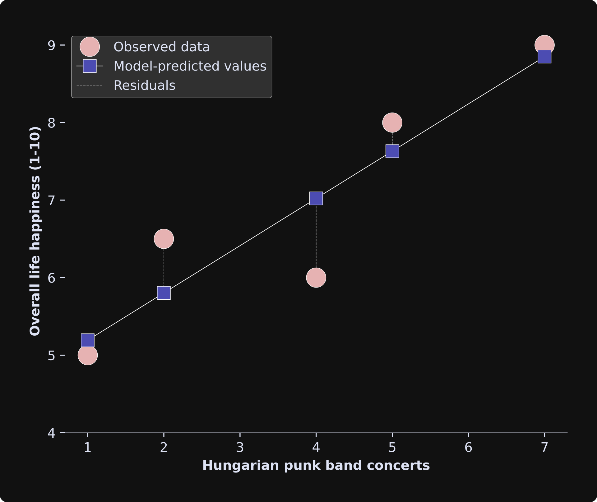
The predictions are pretty decent. Not perfect, but we actually don’t want perfect predictions: The goal of statistical modeling is not to fit the data perfectly, but instead, to fit the data as well as possible with a simple model that captures the essence of the system.
The vertical dashed lines indicate the “residuals” of the model. Those are the estimation errors — the discrepancies between the model predictions and the observed data. Some of the errors are positive, while others are negative. If you square the errors, they’d all be positive-valued, and then we can make sure that our model has the least squared errors. Least squares.
So that’s the linear algebra solution to least-squares. Visually, the results look compelling. But how do we know that the linear algebra solution gives us the least squares?
Keep reading 😉
Least-squares solution (calculus)
The linear algebra equations give us a unique solution, but don’t prove that it’s the best solution. For that, we can approach the regression problem from an optimization perspective: The goal is to get the predicted values as close as possible to the observed data values, which means to minimize the residuals. Let’s start by modifying the equation to put the predicted and observed data on one side, and the residuals (indicated using the Greek letter epsilon 𝝐) on the left-hand side:

The notation || ⋅ ||2 is called the “squared vector norm” and is computed as the sum of squared elements of the vector. Why do we want to optimize the squared errors and not just the errors themselves? Consider that we want the magnitudes of the residuals to be small; we don’t care about their signs. Squaring the residuals makes them all positive, and summing them together gives us one number that reflects the overall magnitude of all the residuals. If we just minimized the errors, we’d get 𝜷 values that push the errors towards -∞, and if we minimized the absolute values instead of the squares, then the derivative gets a bit trickier.
Now for the optimization. The goal is to find the 𝜷 that minimizes ||𝝐||2. In other words, find the solution that gives us the least squares. This can be mathematically expressed as the following:

If you’ve taken a calculus course, you will recognize the form and the solution to this optimization problem: set the derivative to zero and solve for 𝜷.
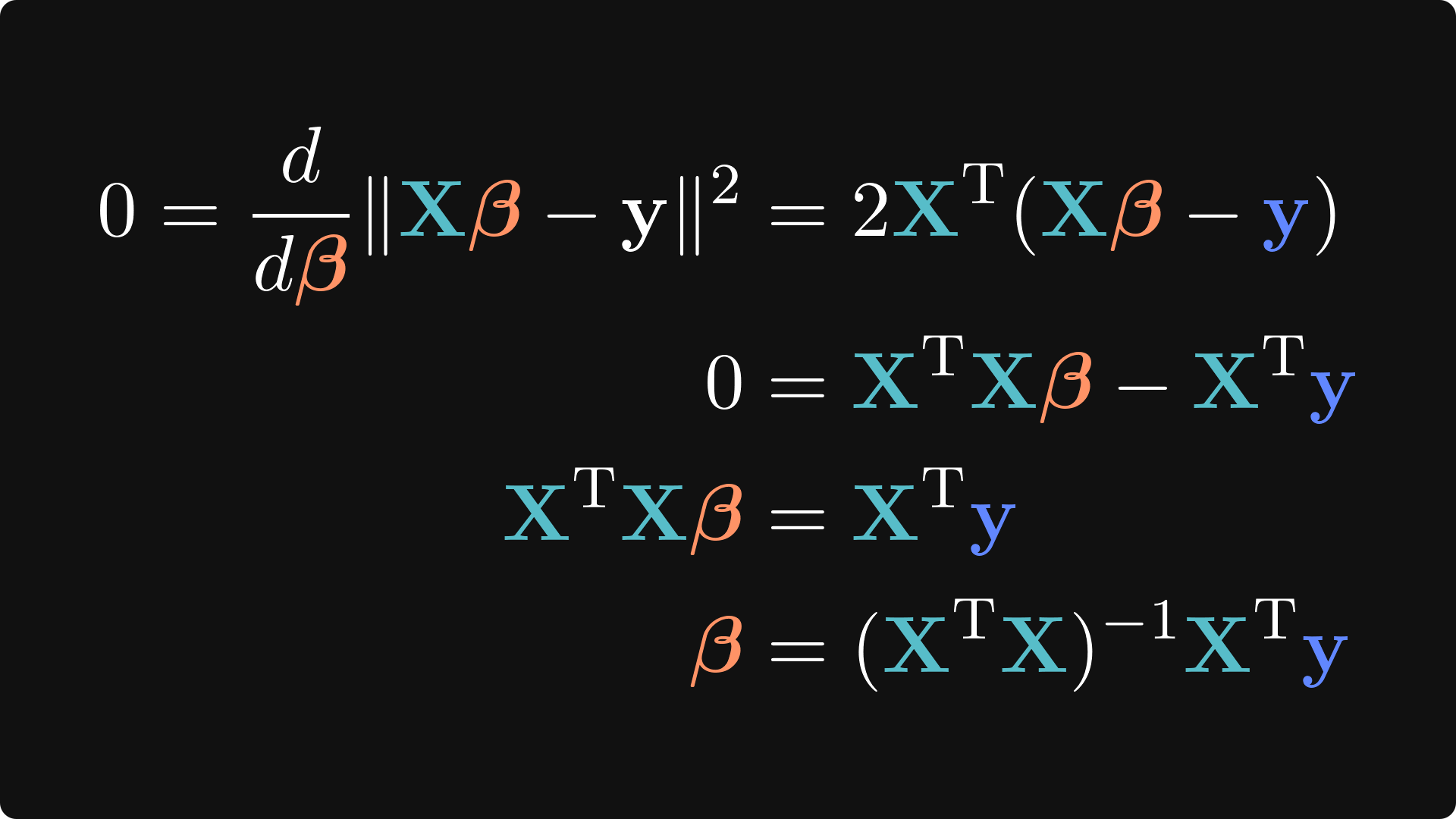
If you’re unfamiliar with matrix derivatives, then don’t worry; you don’t need to fully understand the calculus to understand, or successfully apply, regression models. The upshot is that we defined the objective function as the 𝜷 that minimizes the sum of squared residuals, and the result was the same as what we obtained from the linear algebra approach. This proves that the left-inverse method isn’t just a solution; it’s the best possible solution. (Note for the advanced mathematicians: technically, there is more to this proof, for example, proving that the equation is convex and is a minimum, but I won’t get into those details here.)
Meta-comment: We started from two completely different perspectives, different goals, and different branches of mathematics, and yet ended up with the exact same solution. That is a stunning example of convergence in mathematics.
That’s it for Part 1!
I hope you found this post interesting and elucidating! And I hope you’re excited for Post 2, in which you’ll learn more about residuals, evaluating model goodness-of-fit, and how to create an infinite amount of data to build real intuition about least-squares model-fitting.
If you’d like to learn more from me (an ex-neuroscience professor, current independent educator), please consider subscribing to my Substack, taking my online video-based courses, and checking out my books.
 | A guest post by
|
Dear teacher, thank you for the least-squares article! However, .ipynb files are quite inconvenient to run from the command-line. While you may use jupiter or pycharm, a majority of people don't. It would be very helpful to include .py files along with the .ipynb files so those that use a text-editor and command-line won't have to go through the trouble of copy/pasting (so 90's) just to be able to work along through the problem. Further, the _{2,3,4}.ipynb files are not pretty-print json, so they are obfuscated for all practical purposes. (yes, we could parse it with jq, but that's beyond most substack readers) Think about your friendly Linux students :)
There is one constraint we have to meet det(X^T * T) != 0