

Quick note: there’s a huge 33% discount for my Mathematics of Machine Learning book on Amazon. If you wanted to get a copy, don’t miss out:
Also, if you liked this post, please consider supporting me with a paid subscription. It’s $100 a year, or $10 a month, and in return you get well-researched machine learning/mathematics deep dives such as Machine Learning is Not Just Statistics, Matrices and Graphs, or Vectorization in Theory + Vectorization in Practice.
Your support makes it possible for me to write these high value, high signal posts.
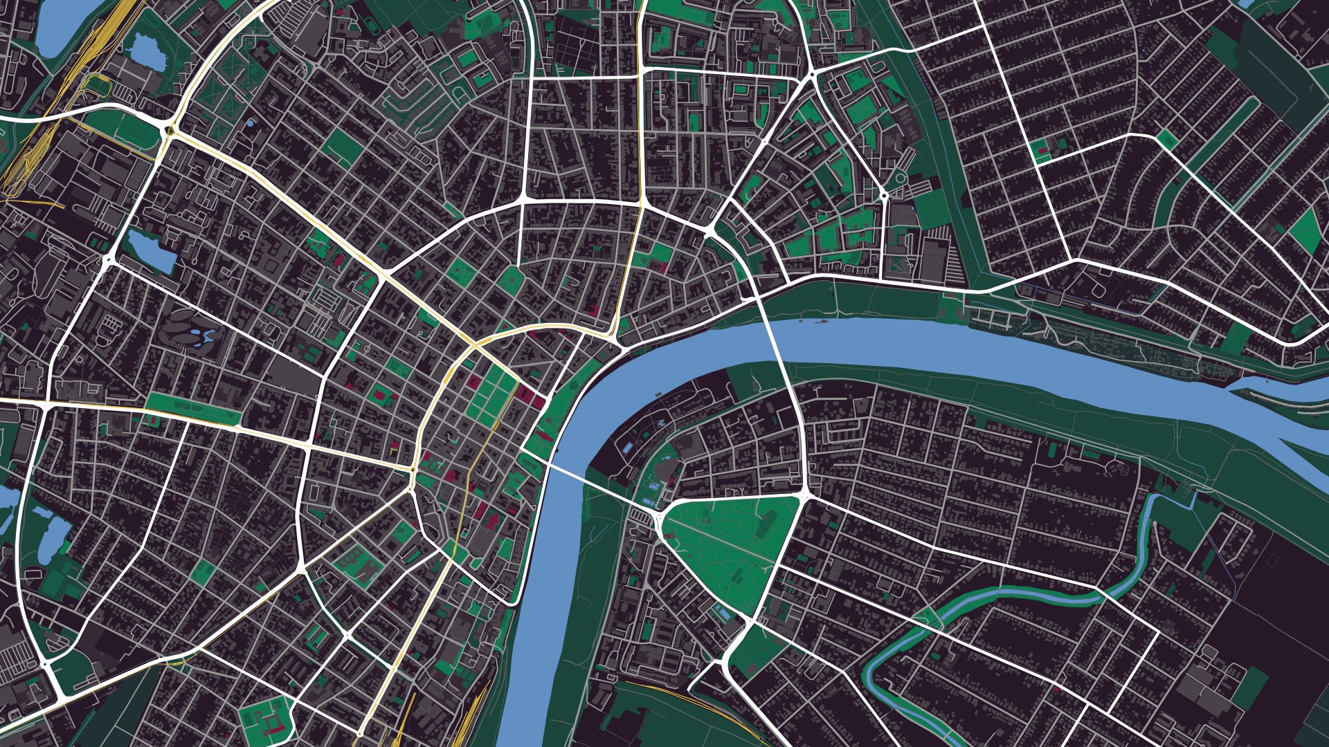
This is my hometown, split into two parts by a river. There are only two bridges connecting the two halves, and a traffic accident on one bridge creates a wave of traffic jams, rippling through the entire city.
To understand why, let’s strip away all the details: the buildings, the river, the parks, the entire layout. Everything except the streets and intersections. Each intersection becomes a dot, and each street segment becomes a connection between them. We’ve thrown away most of the map but kept what’s essential: what connects to what. That’s a graph.
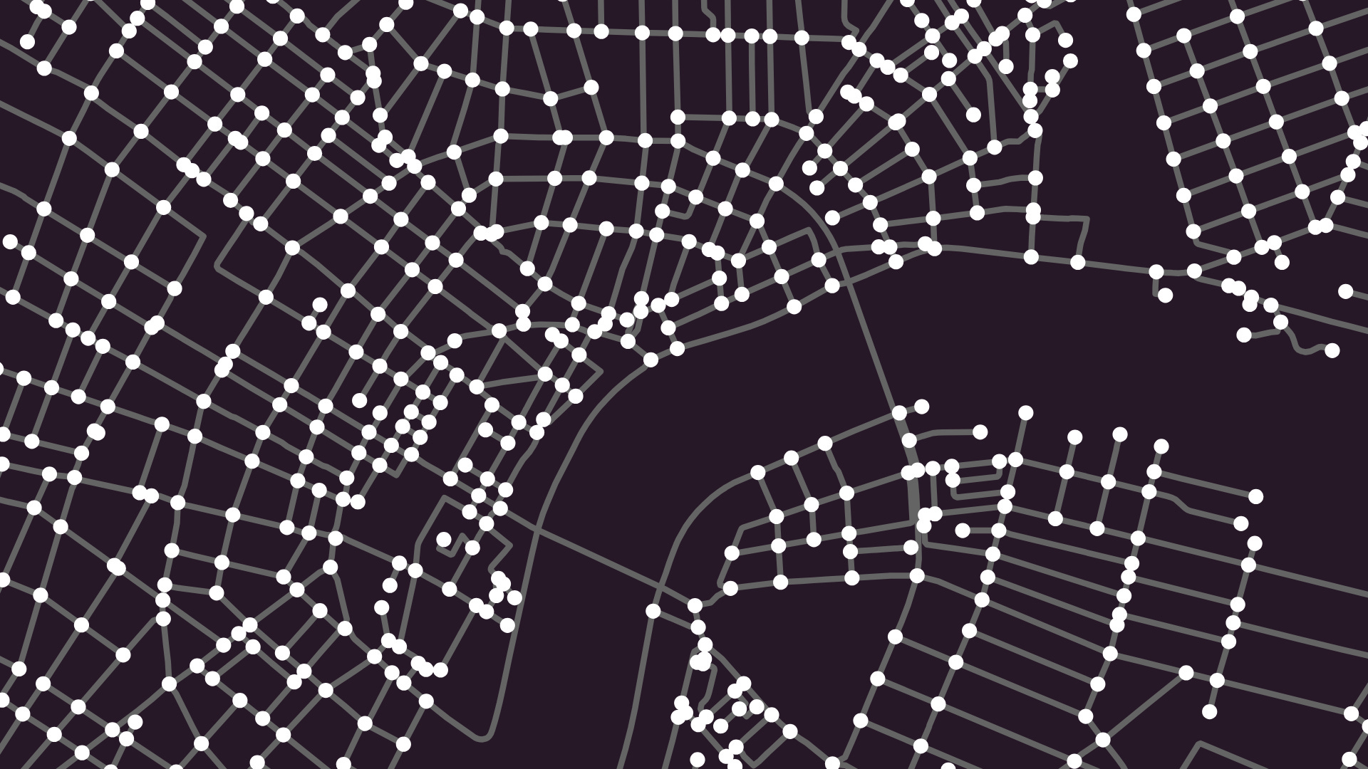
Traffic is now a walk on the graph, flowing from node to node along the edges. Close one bridge, and traffic crossing the river has to use the other. If it can’t handle the extra load, the traffic freezes. Close both, and the two sides become disconnected.
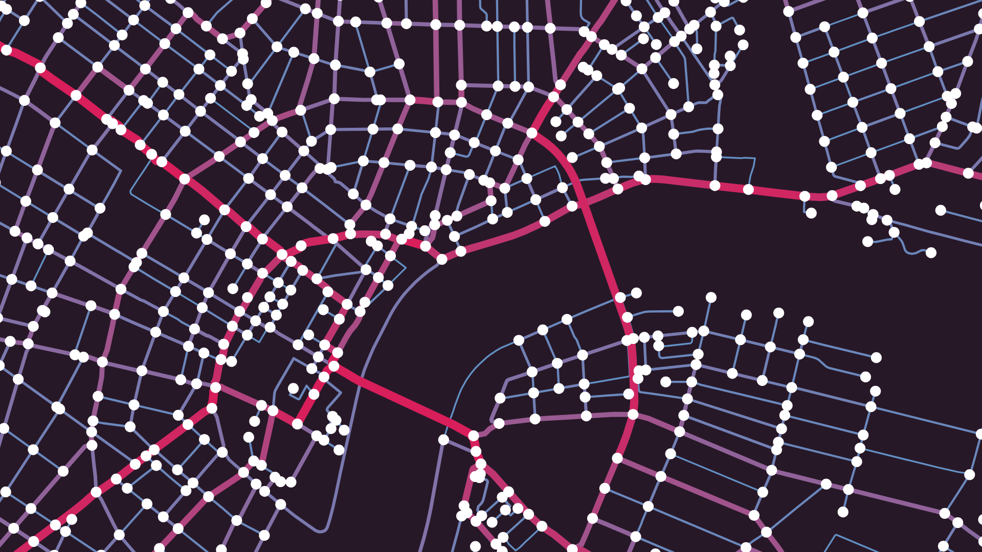
It’s easy to see that the bridges are important, but which other connections matter more than they seem? If we highlight the streets that appear on many shortest paths, the traffic arteries of my city emerge. When I first saw this, it felt like magic. It’s really not; it’s just graph theory, and we’ll learn all about it soon.
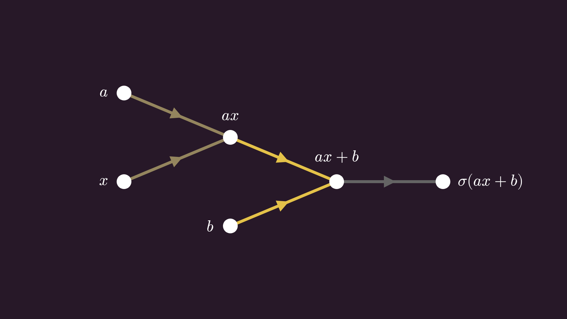
Graphs are just dots and lines, but with enough dots and lines, we can model almost anything. Mathematical expressions, where nodes represent variables and edges represent computations.
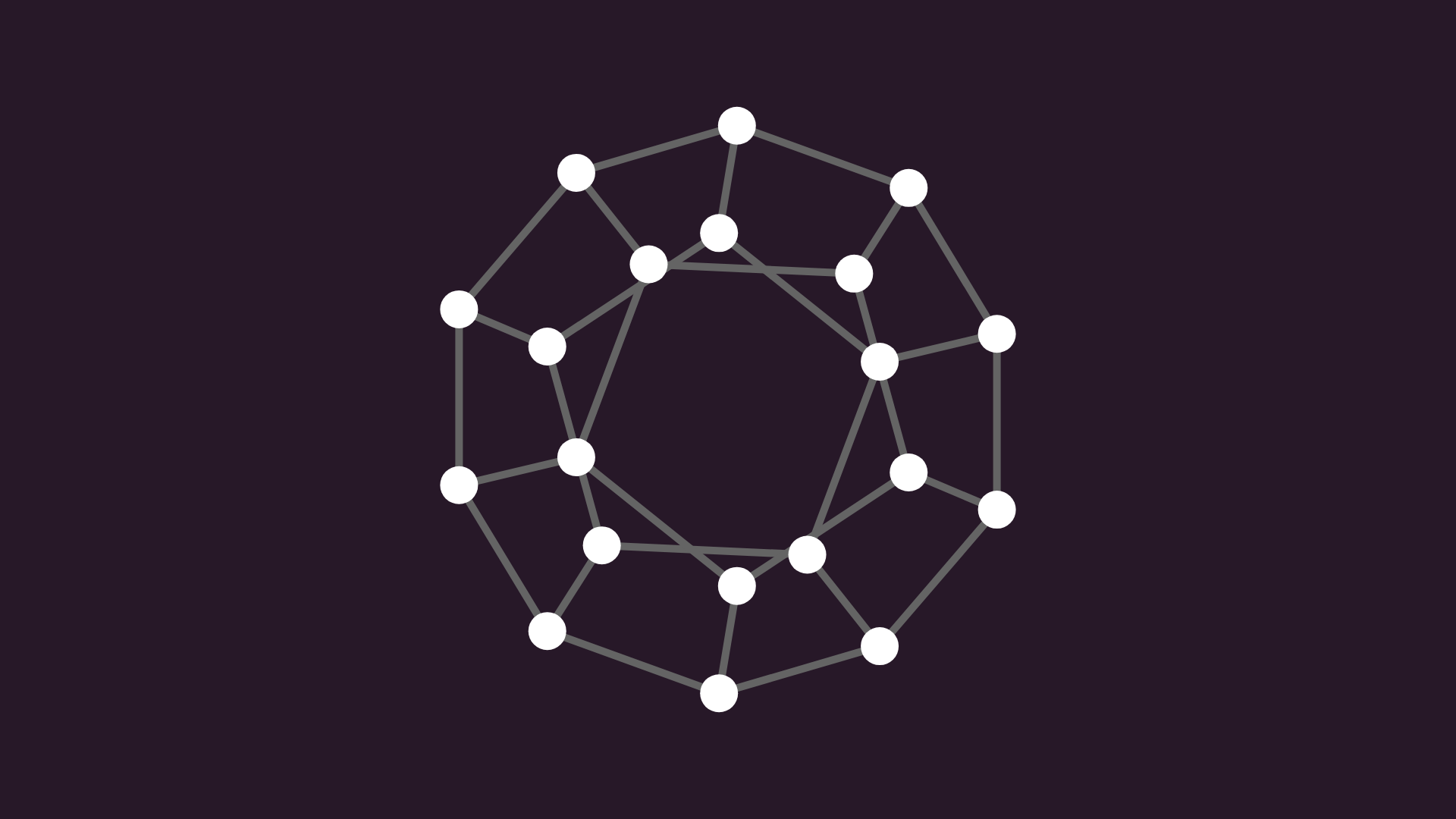
Or geometric shapes, where nodes represent vertices, and edges border the faces.
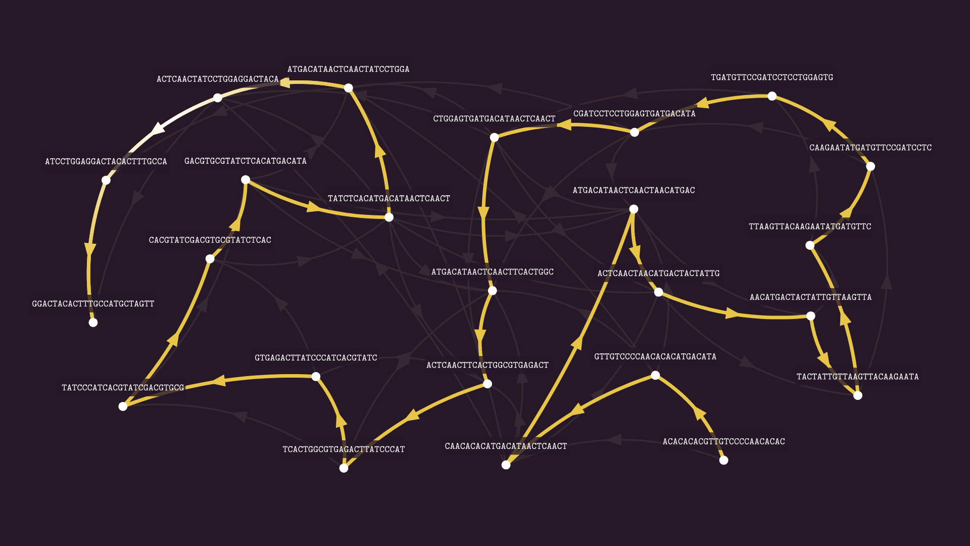
Or DNA fragments, assembled into a full genome sequences via graph algorithms.
Graphs are everywhere, and graph theory gives us a powerful language to work with them. In this video, we’ll build this language step by step and use it to analyze traffic, find optimal paths, assemble genomes, and much more. But let’s start at the beginning. What is a graph?
Video version of the post:
What is a graph?
Mathematically speaking, a graph is a set of nodes and edges. The simplest way to represent graphs is by drawing dots and lines.
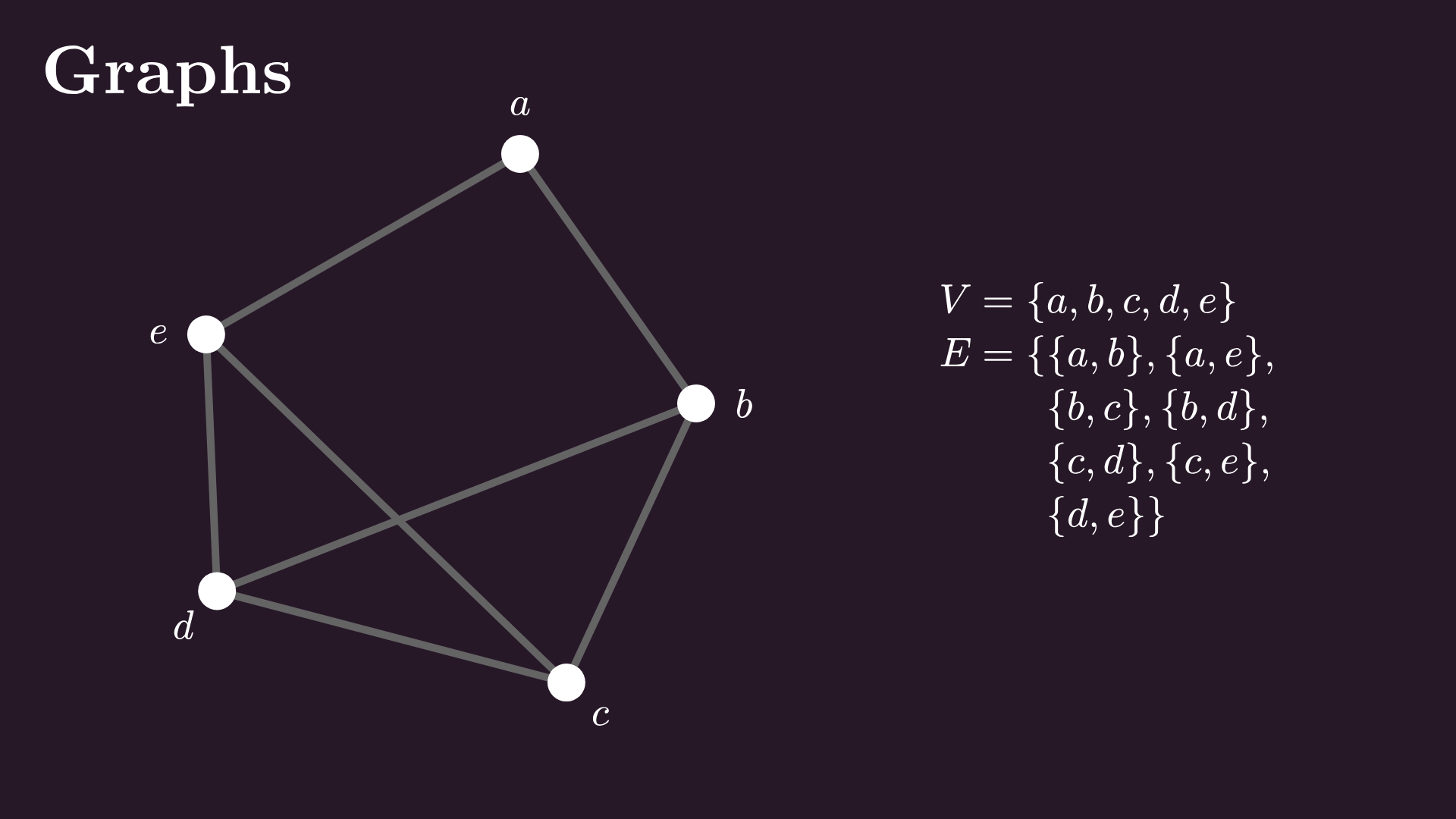
Each edge is a two-element subset of vertices. This is called a simple graph. We’ll add loops, weights, and directions to our edges later, but for now, let’s stick with the most basic version.
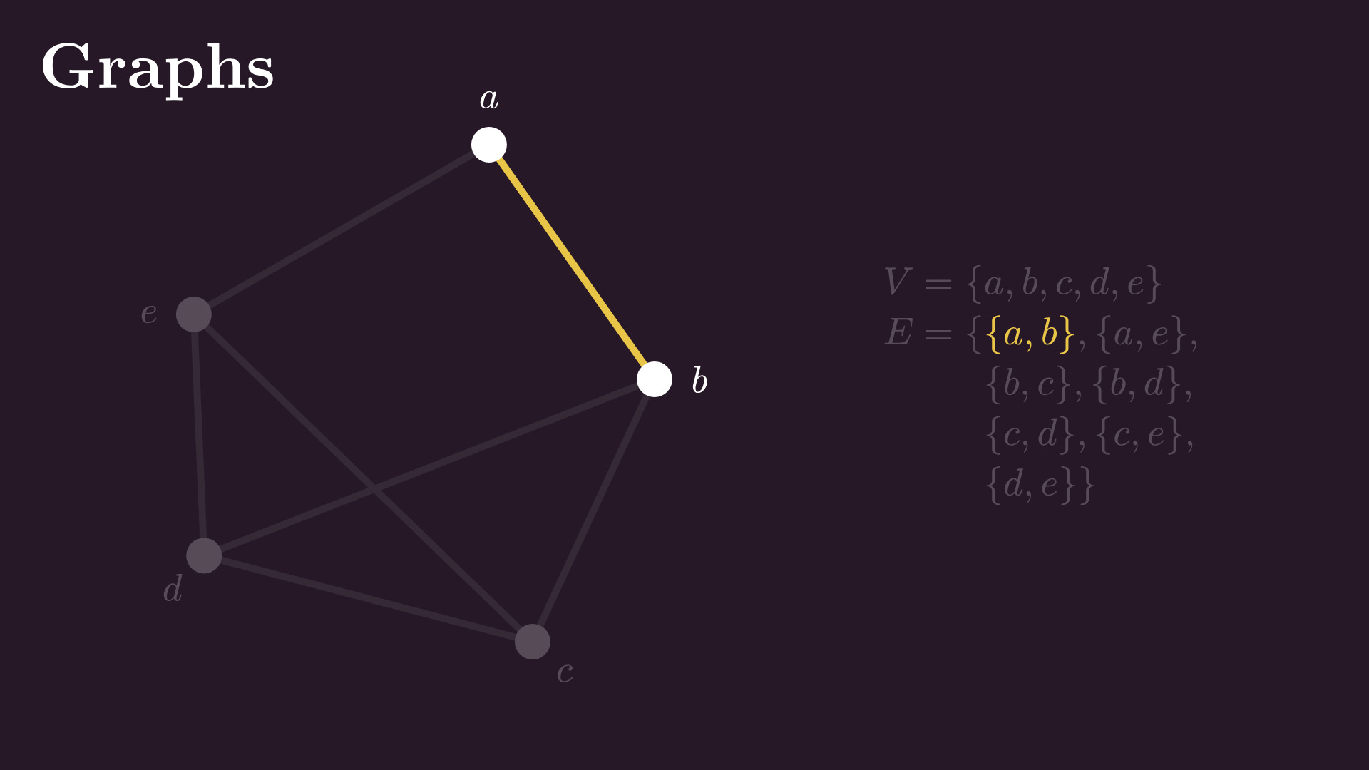
The dots-and-lines diagram you see is called a drawing of the graph. (Or a two-dimensional embedding, if you want to be fancy about it.) It’s not mandatory to only use straight lines for the edges; we can bling them out as much as we want.
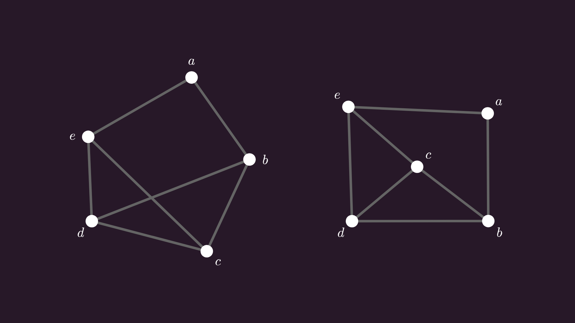
You should be careful not to identify a graph with its drawing, as there are infinitely many ways to draw the same graph. For instance, these two drawings represent the same graph.
In this case, when two drawings represent the same underlying graph structure, we say that the two graphs are isomorphic.
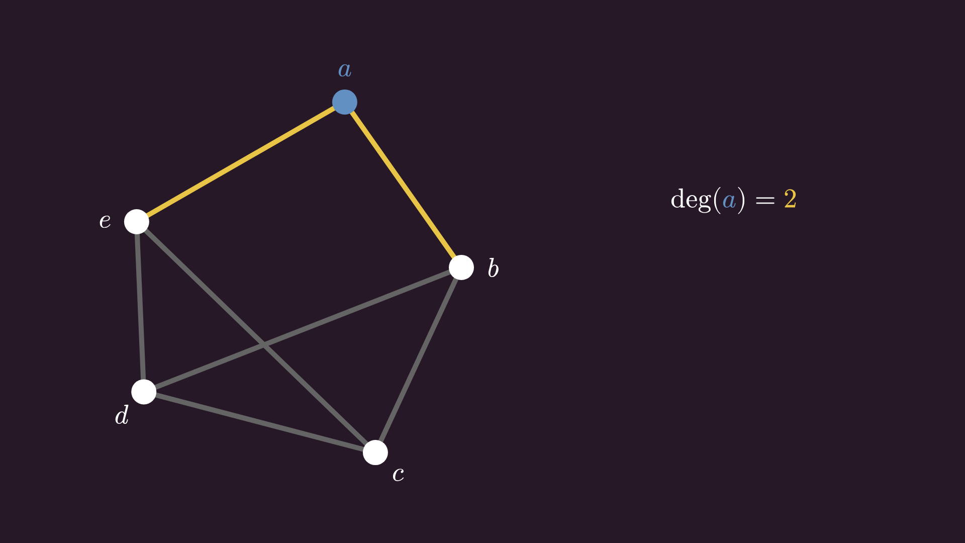
An important property of a node is its degree, that is, its number of incident edges.
In our example graph, node a has a degree of two, node b has a degree of three, and so on.
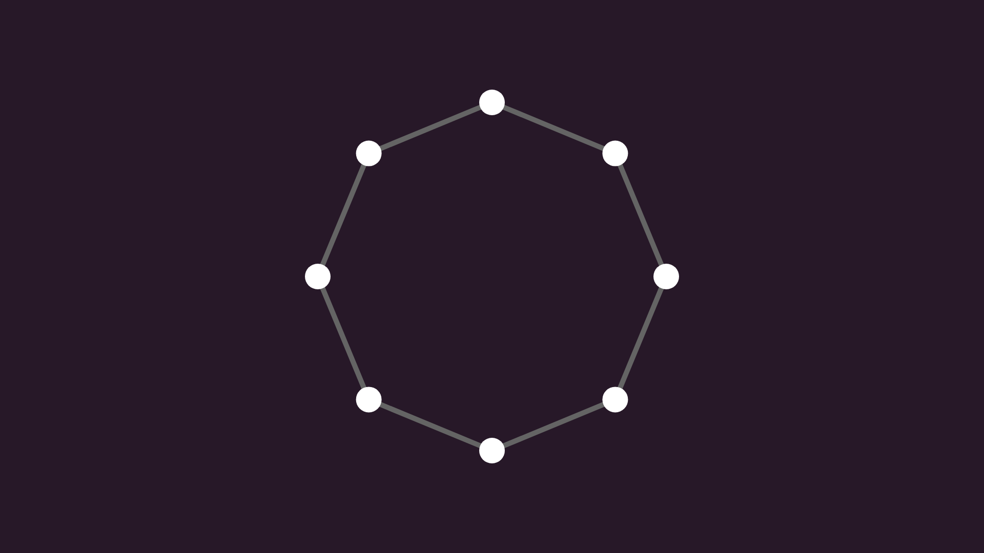
A node’s degree gives valuable local information about the structure of our graph, but the degrees alone are not enough to reproduce the graph. For instance, in this graph, every node’s degree is two. If we break this circle into two, the degrees don’t change, yet the two graphs are not isomorphic.
Walks and paths
Speaking of local information: let’s move on to the global structural properties of graphs.
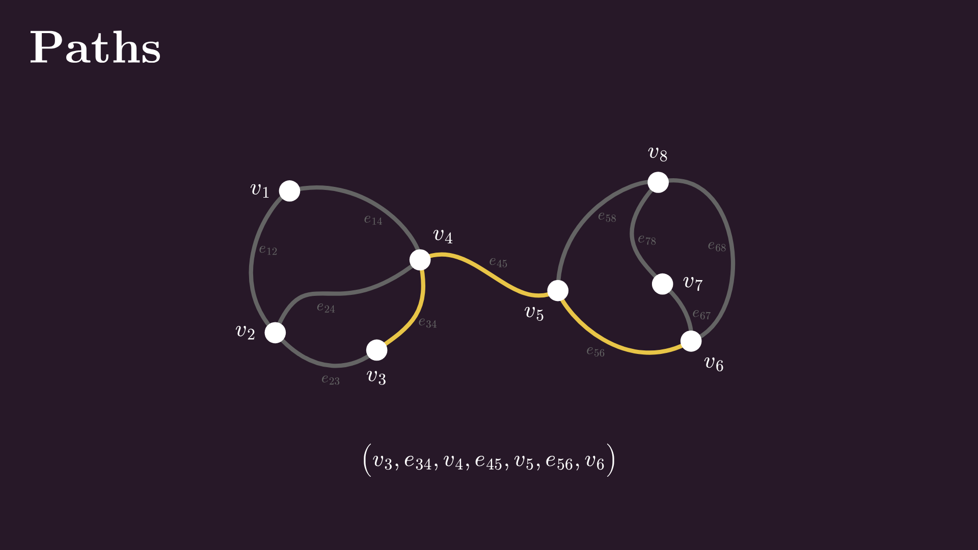
You can think of an edge as a step from one node to another. Chain multiple steps together, and you have a walk.
Mathematically speaking, a walk on the graph is an alternating sequence of nodes and edges. If we label all edges and nodes appropriately, we can visualize the process.
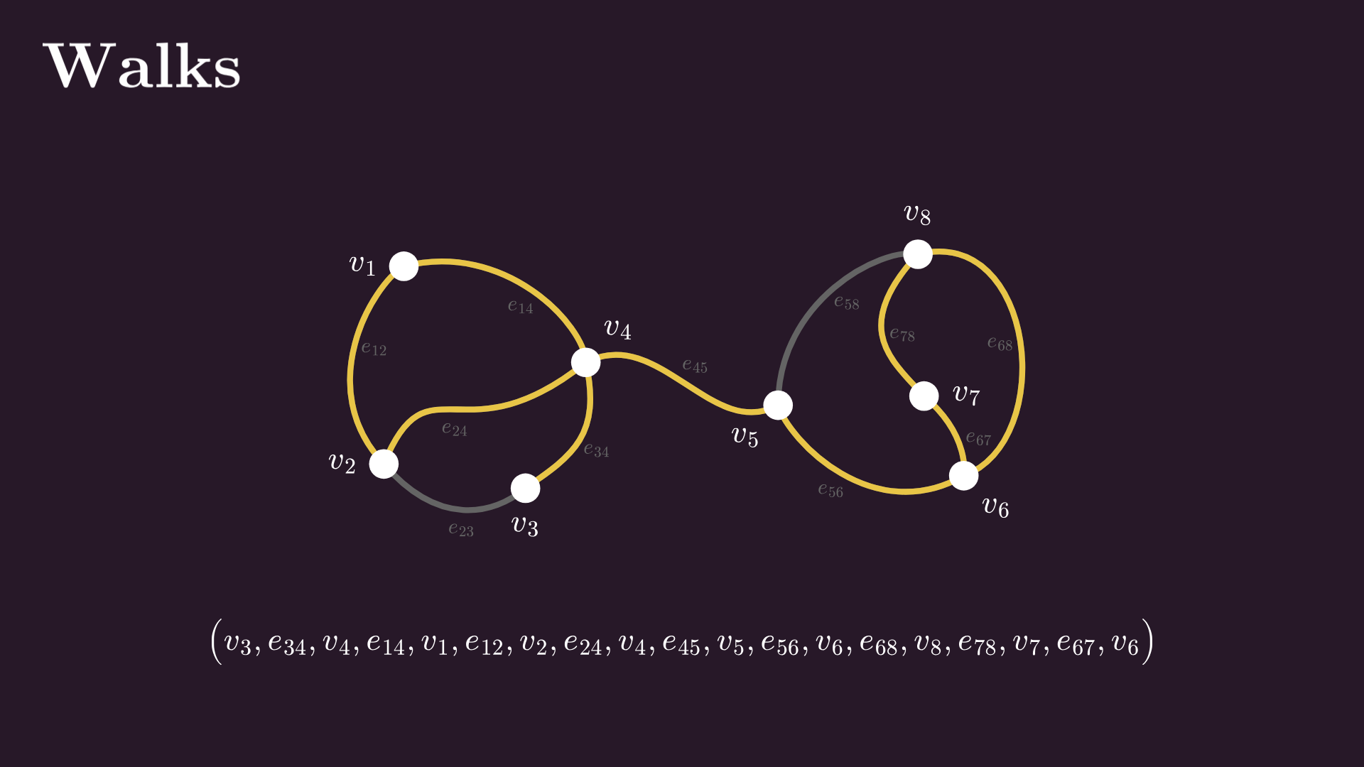
A walk can have repeated nodes and edges, and as we often only care about the first and the last nodes, we trim the walk to get rid of those repetitions. In this example, these two loops are just unnecessary round trips, so we can just clip them and still reach our intended destination.
A walk without repeated edges or nodes is called a path. We can always eliminate repetitions from a walk like we’ve just seen, so we’ll often use paths instead of walks.
Why are paths interesting? First of all, the study of paths launched graph theory itself, when Euler wanted to take a walk in Königsberg that crosses all bridges exactly once.
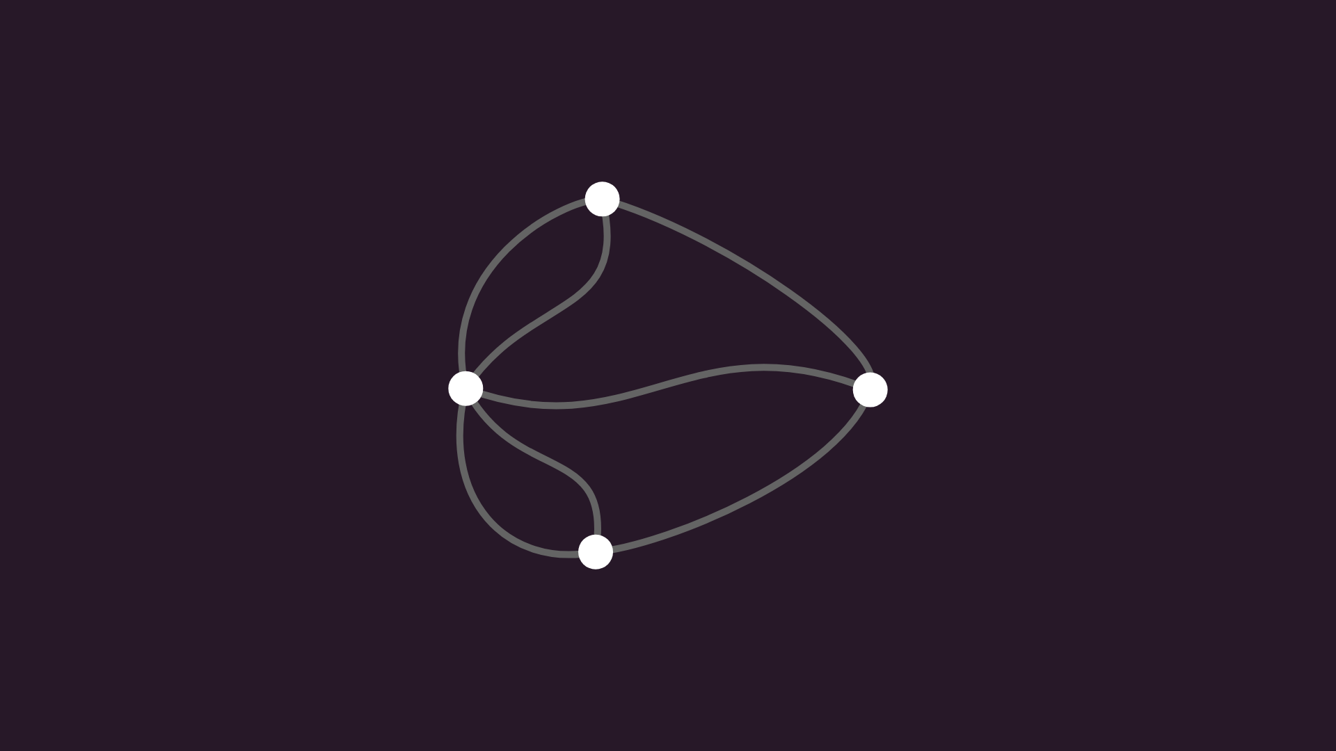
The islands and bridges of Königsberg can be represented with this graph. As it turns out, Euler’s path is impossible on it, but as a positive side effect, the field of graph theory was born. Three hundred years later, it’s everywhere in our lives.
Connectivity
Let’s get back on track. Paths provide us with a way to study the global structure of graphs. When there’s a path from node a to node b, we say that b is reachable from a.
This is an equivalence relation: 1) it is reflexive, meaning every node is reachable from itself; 2) it is symmetric, meaning that if b is reachable from a, then a is reachable from b; and 3) it is transitive, meaning that if b is reachable from a and c is reachable from b, then c is reachable from a.
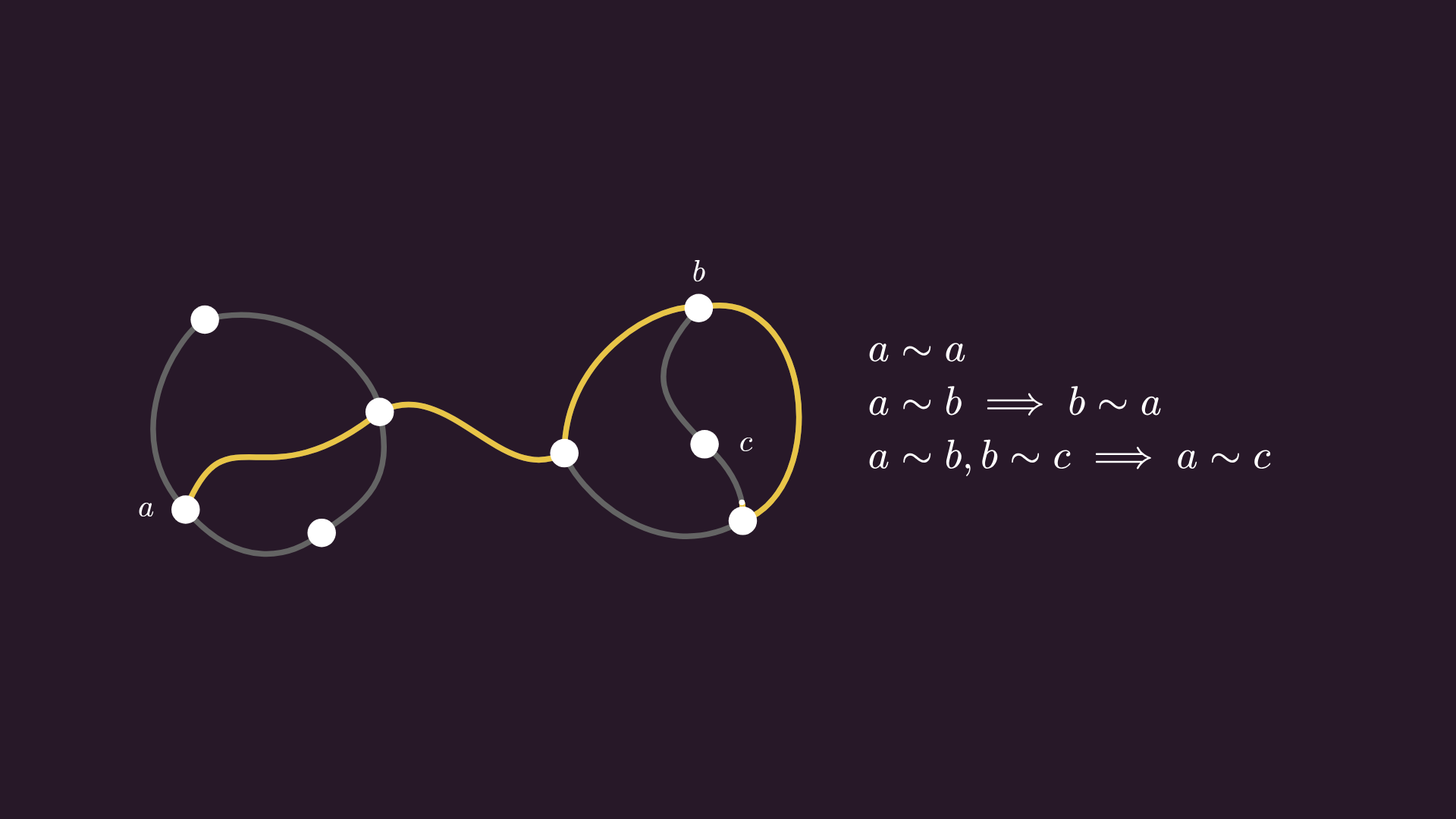
We say that a graph is connected if every node can be reached from every other node. Because reachability is an equivalence relation, it is enough to find a single walk that connects all nodes, like in this example below.
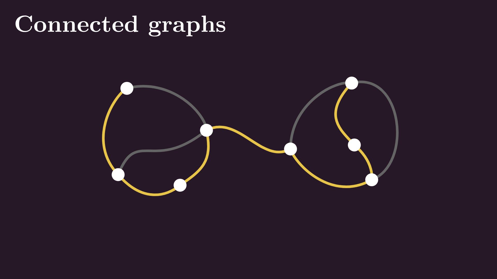
However, if we remove that edge in the middle, the remaining graph is not connected anymore. We call this graph 1-connected, or simply connected.
We can push this idea even further. For example, the graph of my hometown falls apart when we remove two edges (the ones representing the two bridges).
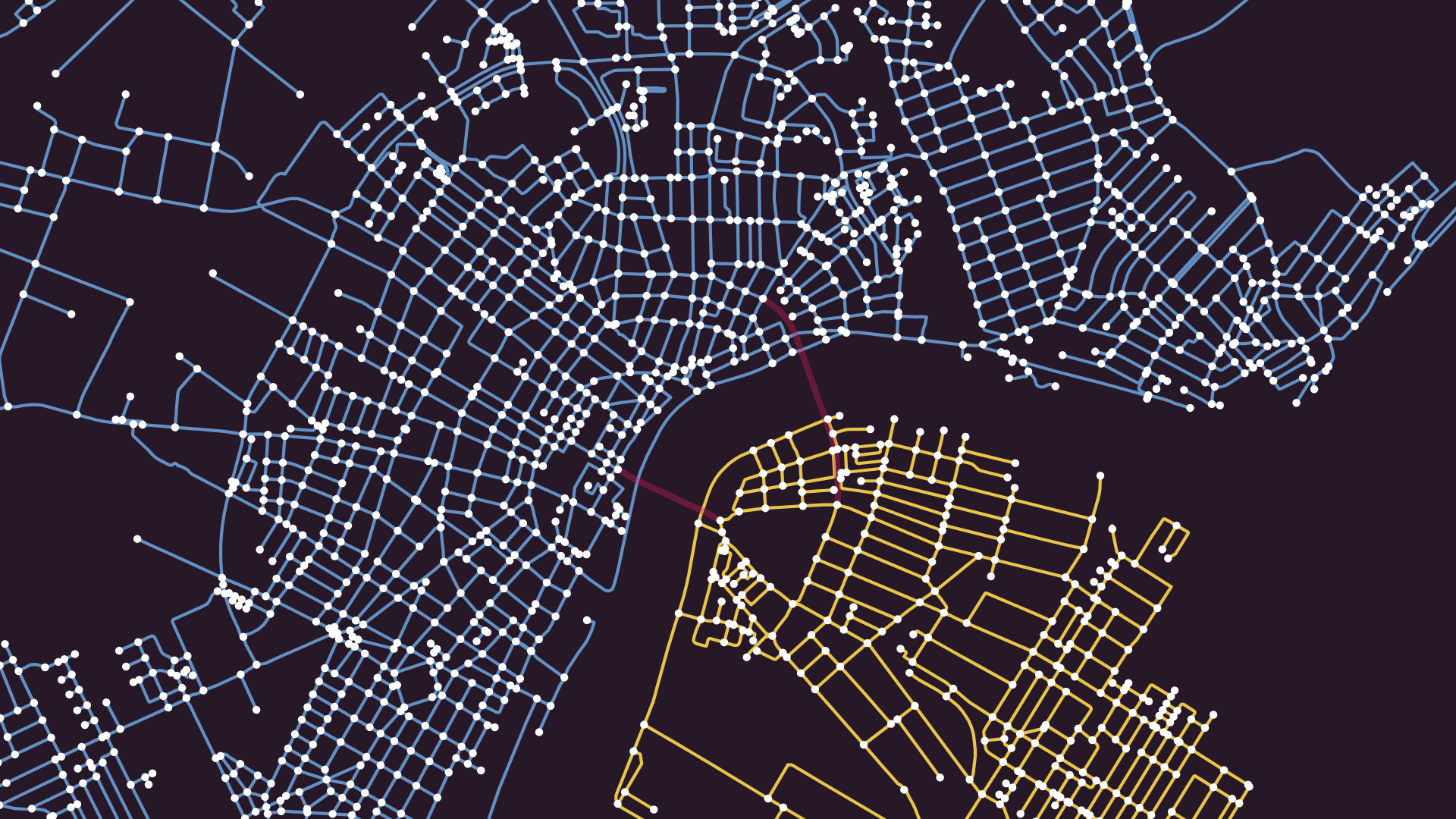
But how to actually find these components in practice? Here, you can just take a look at the drawing, but there are two issues. First, good luck doing that on a large and messy graph.
Search
Second, think about how graphs are represented inside computers. Algorithmically speaking, we only see a list of nodes and their neighbors.
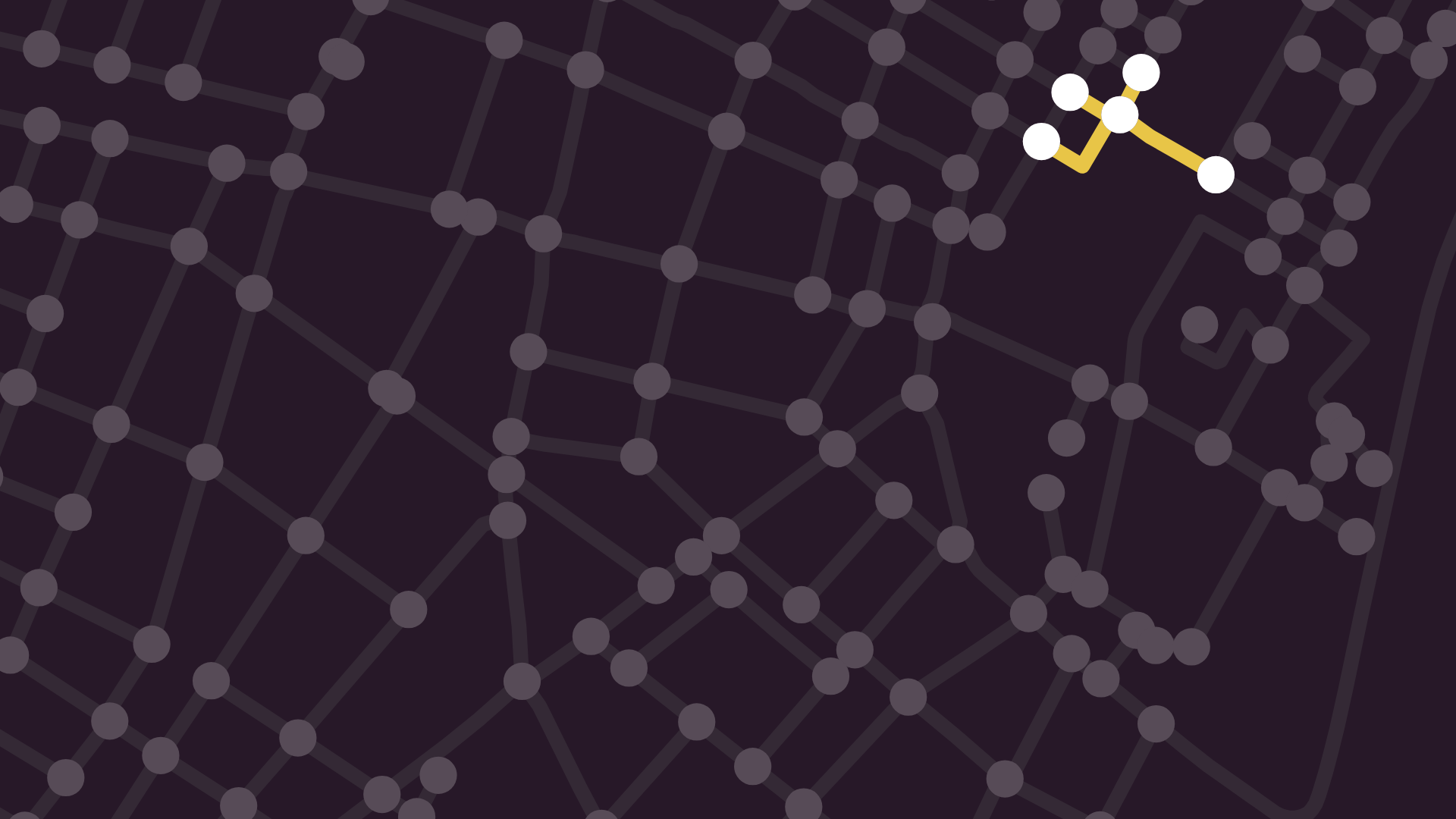
In practice, searching for a path feels like navigating a labyrinth with a blindfold on, stumbling from room to room, having no idea where the exit is. So, we need a strategy to systematically explore graphs. There are two of them: breadth-first and depth-first.
Let’s start with the first one. Breadth-first search is an iterative approach, exploring a graph layer by layer. First, we pick a starting node, then record all of its neighbors; this is level one. Then, we loop through all the recorded nodes and check their previously unvisited neighbors as well; this is level two. You get the gist: we continue this process until the entire connected component is exhausted.
Notice that as we removed the bridges, our search traversed only one component, which circles back to our motivation: finding the connected components. To find the other ones, we can simply launch another breadth-first search from the unvisited nodes.
Alright, now let’s see the other strategy: the depth-first search.
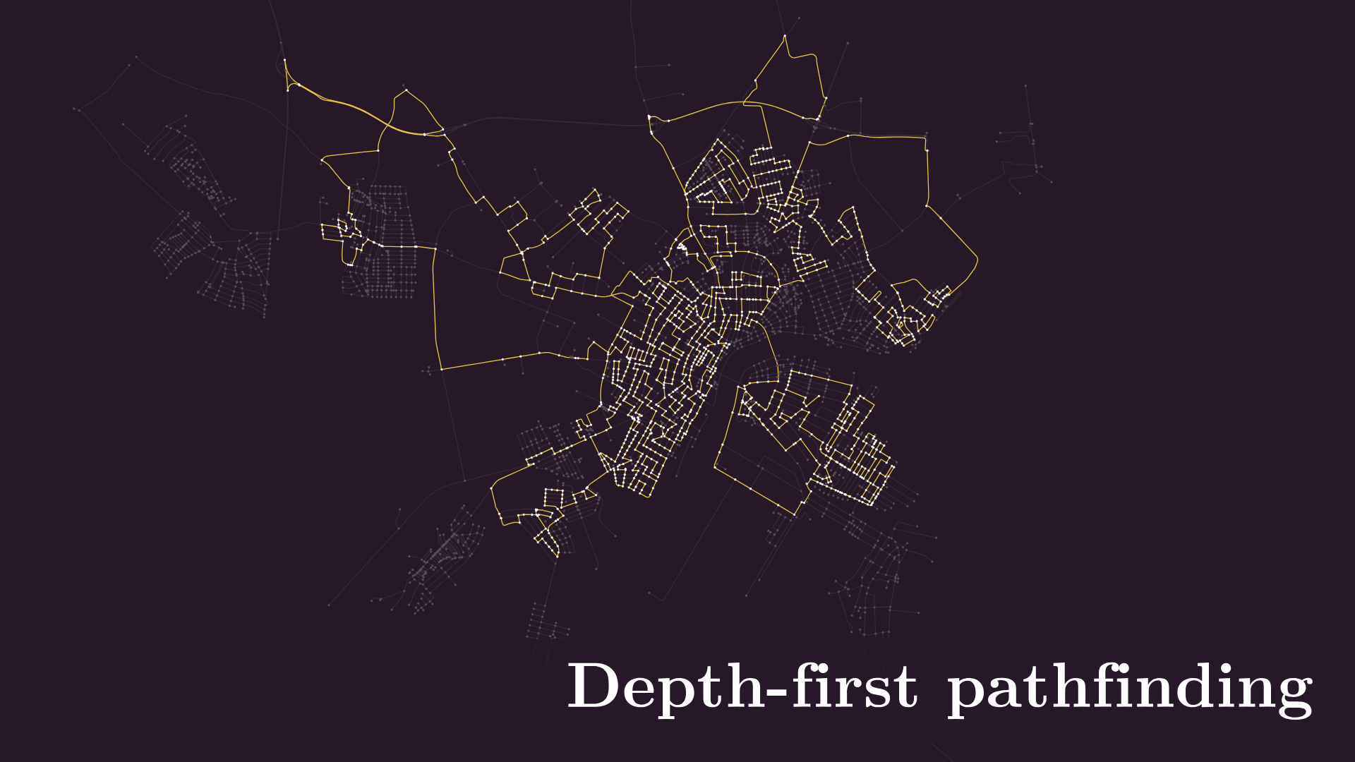
This time, instead of exploring every node layer by layer, we go towards unvisited points as long as we can, until we hit a leaf node or there are no unexplored neighbors. In our city graph, we can imagine this as driving out as far as we can.
When we can’t go forward, we backtrack to the last node until we hit the stopping point again. And again. And again, until there are no more nodes to backtrack to.
Depth-first search also finds only one component, so we can start another one from any of the remaining nodes, like before.
These two strategies are the main ones, but how to decide which one to use? It all depends on the underlying graph and our use case. But before we move on, let’s re-add those two bridge edges, as we’ll need them later.
Let’s say you want to find a path between A and B in the city. If you perform a breadth-first search from A, you’ll get a path with a minimum number of edge traversals.
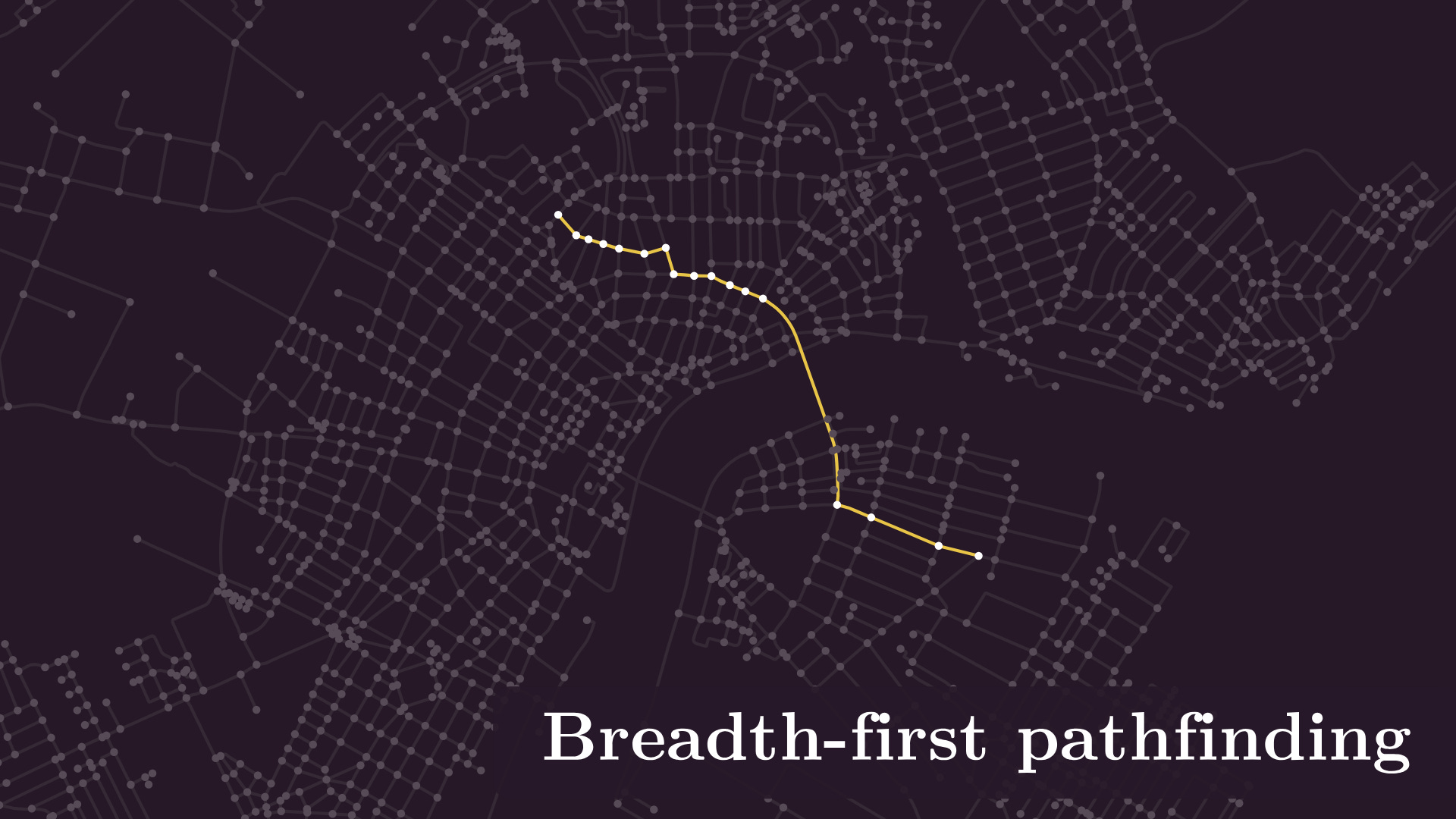
On the other hand, even though a depth-first search is guaranteed to find a path, it might be a very long one. So, breadth-first search usually wins the pathfinding contest.
We’ll return to these two bedrock algorithms later, but for now, let’s move on to another important topic: cycles.
Cycles
Let’s start at the beginning. We say that a walk is closed if it ends where it started.
In turn, walks without repeated edges are called trails. (Trails are not necessarily closed.)
Finally, closed trails without repeated nodes are called cycles, which are one of the most important structures in graphs.
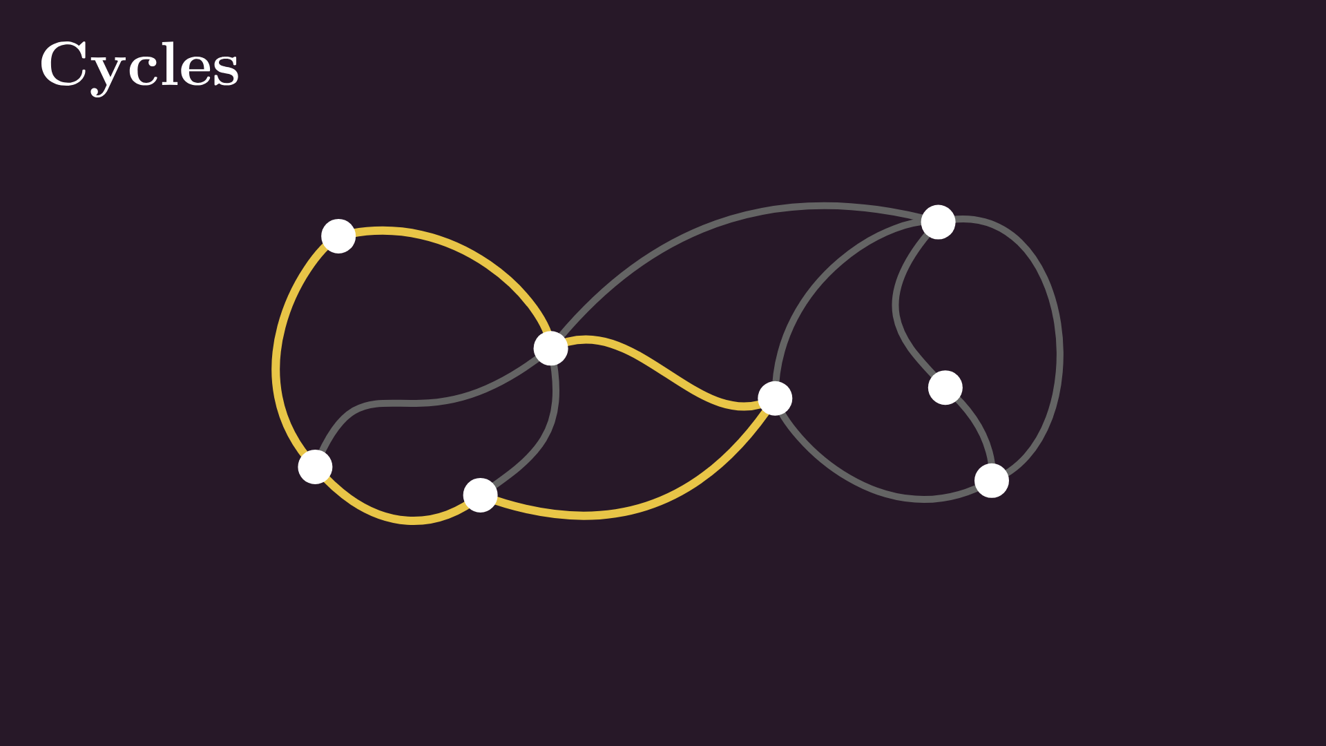
Why are circles important? I like to think of them as structures that make graphs resilient to edge removal attacks: remove any edge on a circle, and the graph stays connected.
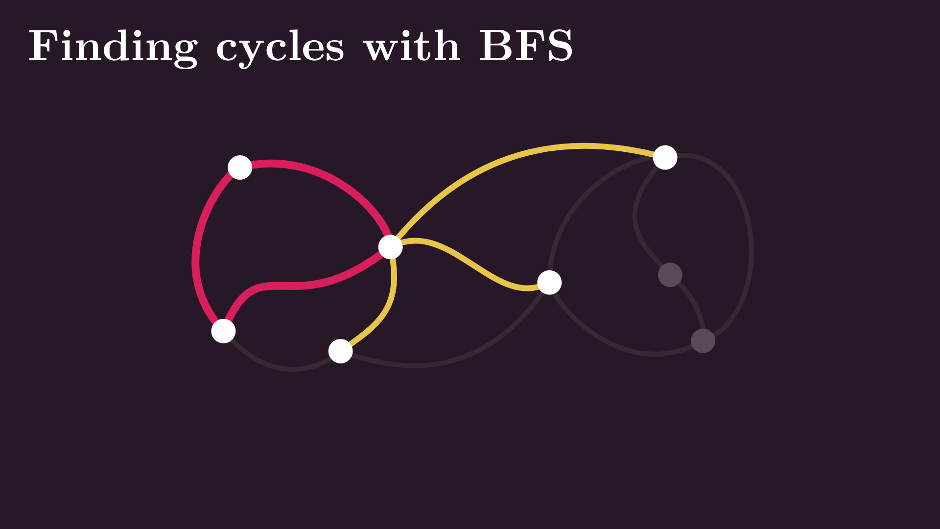
Before we expand on this idea, let’s see how to find cycles in practice. You guessed it: it’s breadth-first and depth-first search. By properly keeping track of visited nodes and their parents, both are capable of finding circles in the graphs. These are the circles found by BFS:
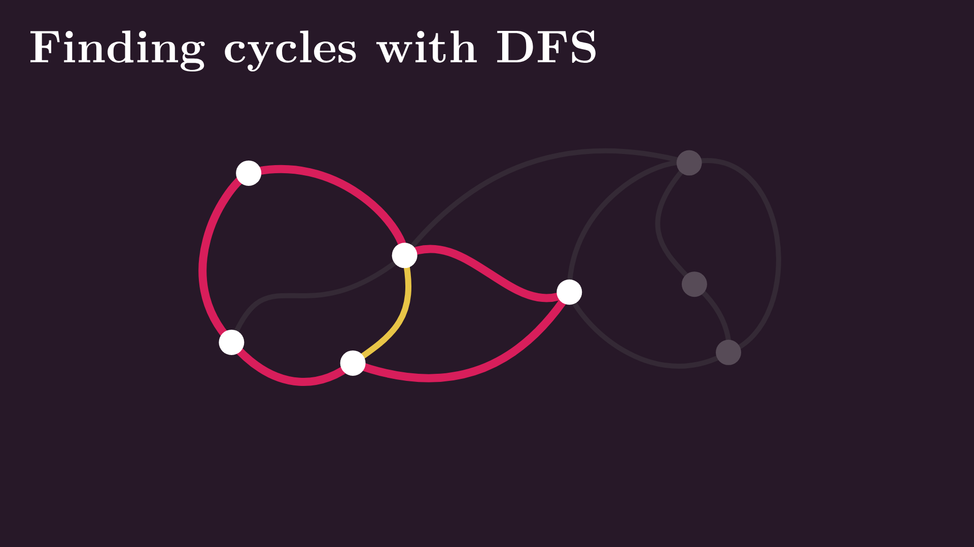
And these are the ones by DFS. One of my university professors used to say that graph theory pretty much comes down to throwing these two search algorithms at any problem, and finding cycles is no different.
Trees
So, again, why are circles important? I mentioned that we like circles because they make the graphs resilient to edge removal attacks, but that’s just one side of the coin. What we don’t like about cycles is that they make paths between two points ambiguous; there are many different paths between these two nodes that are otherwise edge hops away from each other.
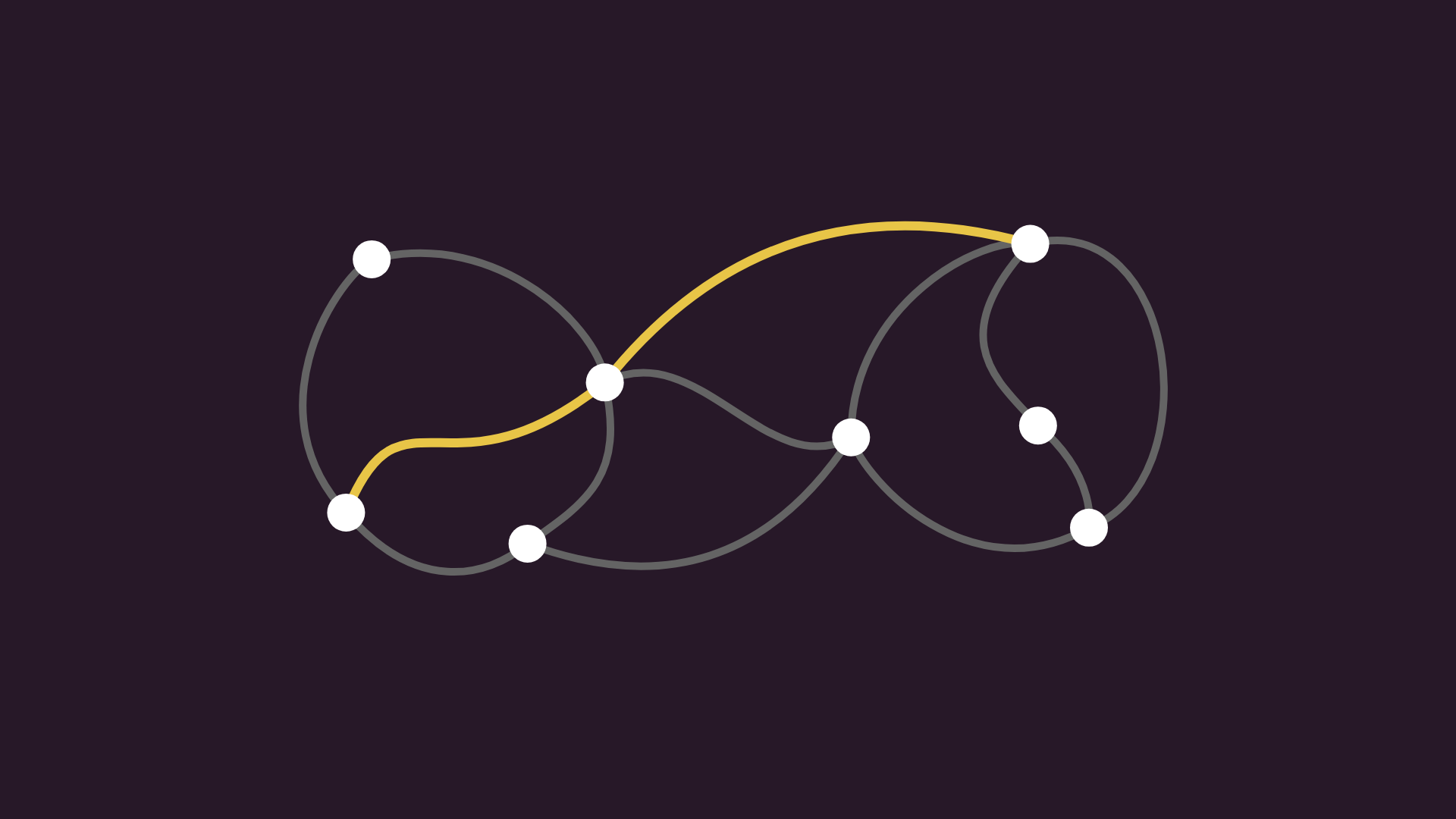
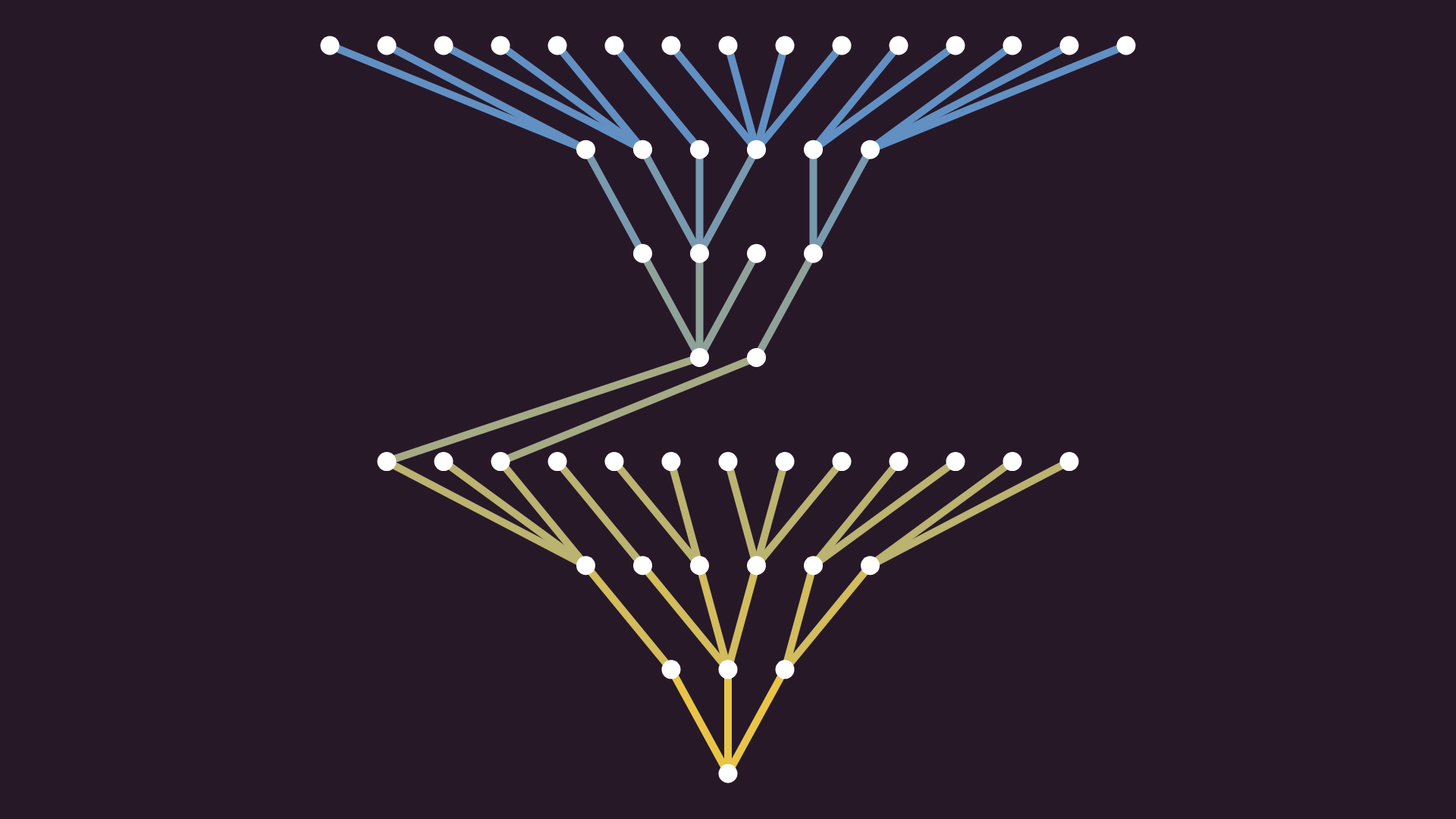
Cycles not only make pathfinding more complex, but they also block hierarchical orderings on a graph. So, connected graphs without any cycles are special. Because of their resemblance, we call them trees.
We love trees. They are simple, beautiful, and have a bunch of useful characterizations. By definition, they are the connected and acyclic graphs, but there are other equivalent definitions.
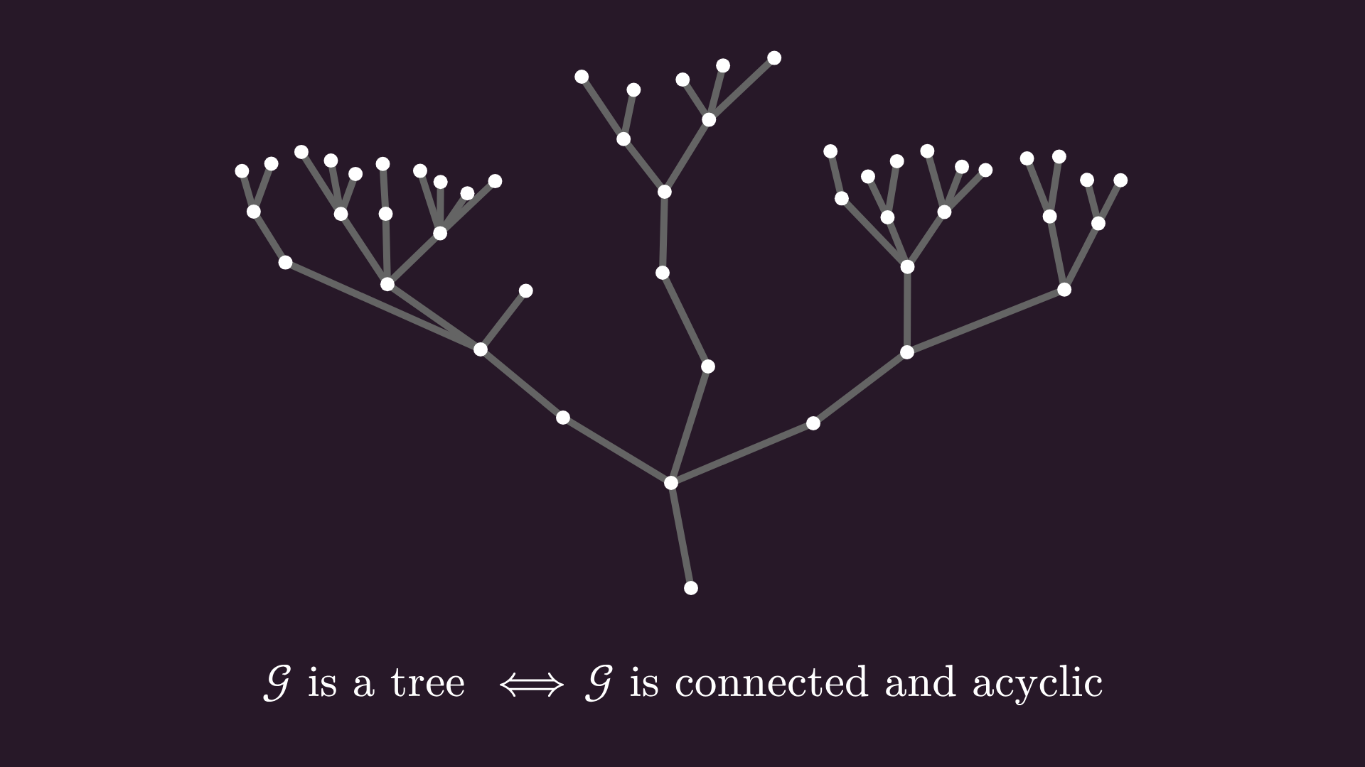
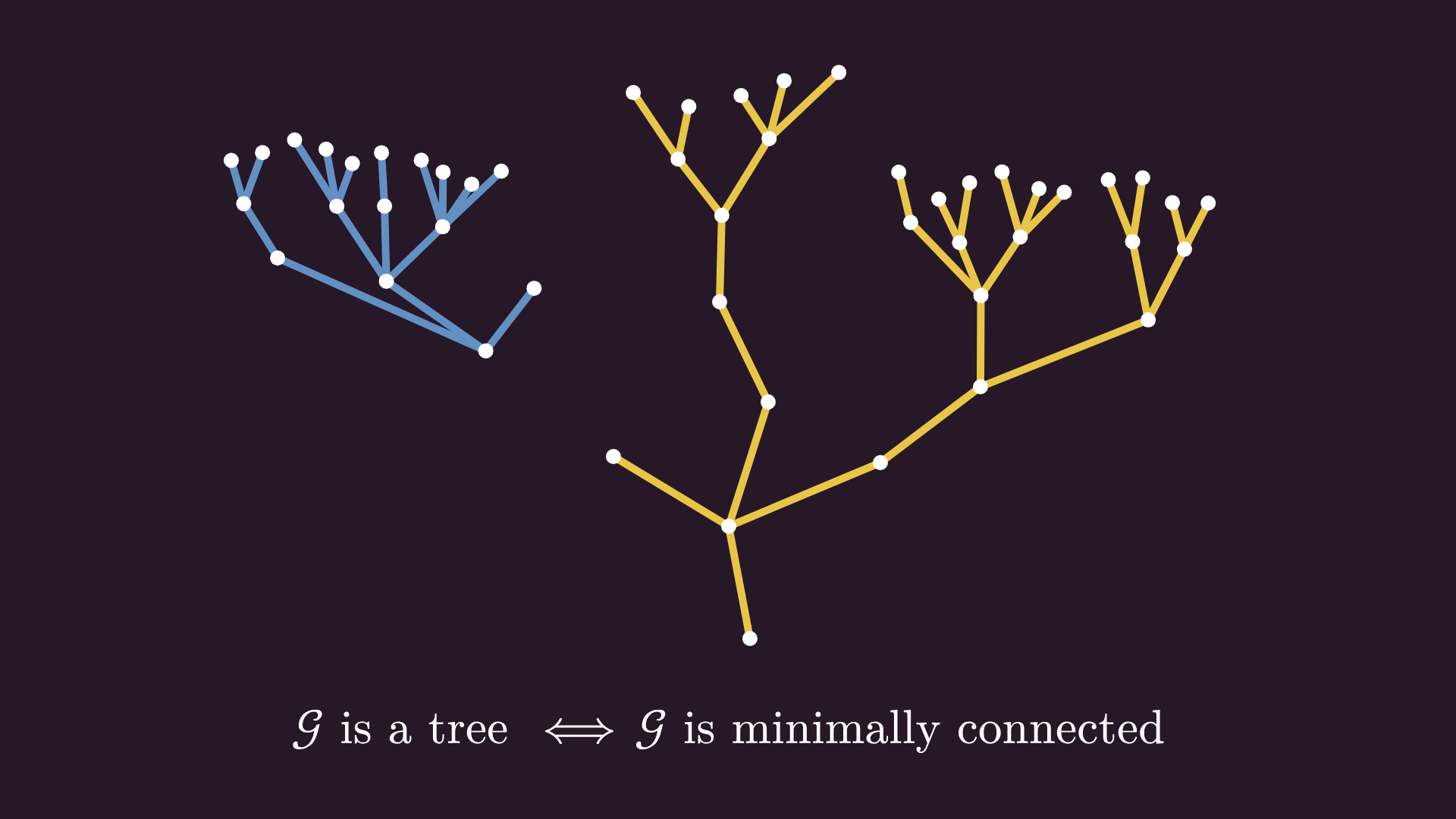
The first one is that trees are minimally connected graphs: remove any edge, and they fall apart into two components. This means that there are no redundancies, no wasted edges. If the graph models a power grid, the tree property means no wasted power lines.
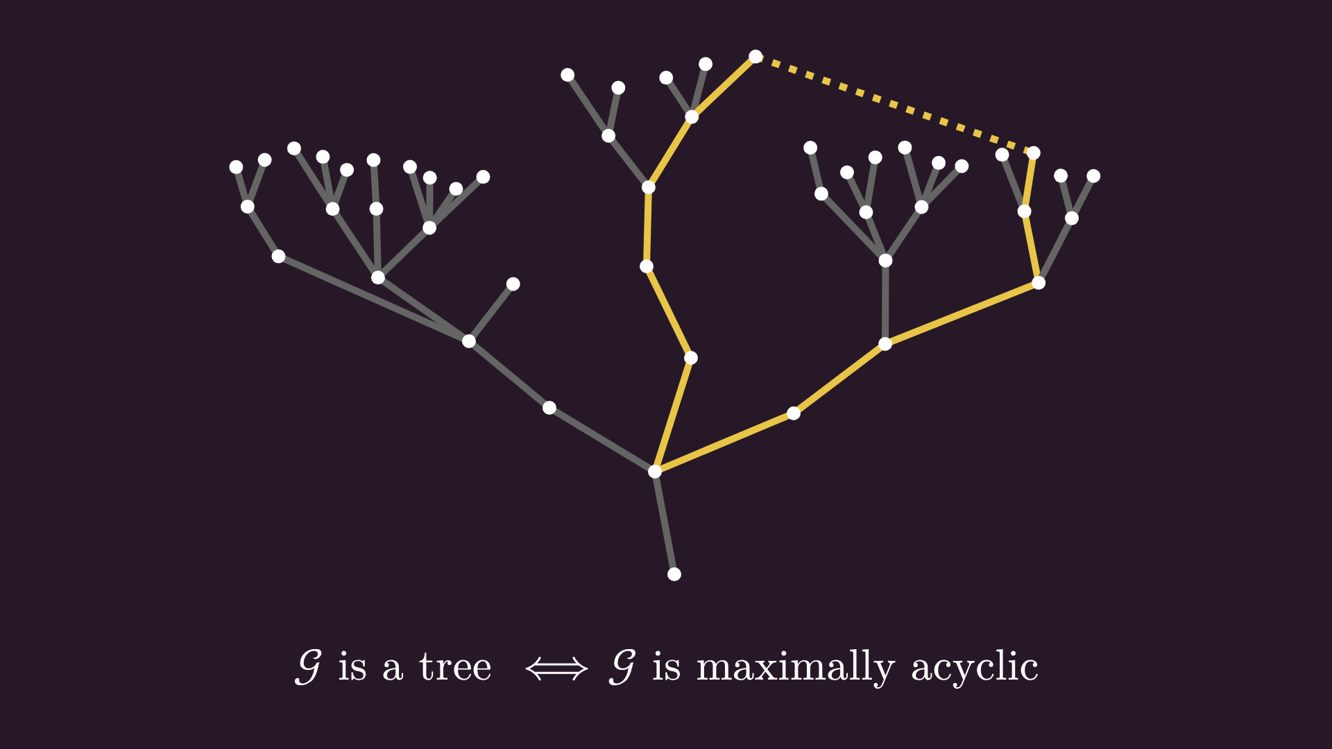
On the other hand, adding any new edge between two existing points creates a cycle. Mathematically speaking, trees are maximally acyclic.
Alright. One last characterization, my favorite one. The acyclic and connected structure is equivalent to having exactly one path between any two nodes: connectedness guarantees at least one path; acyclicity blocks the rest.
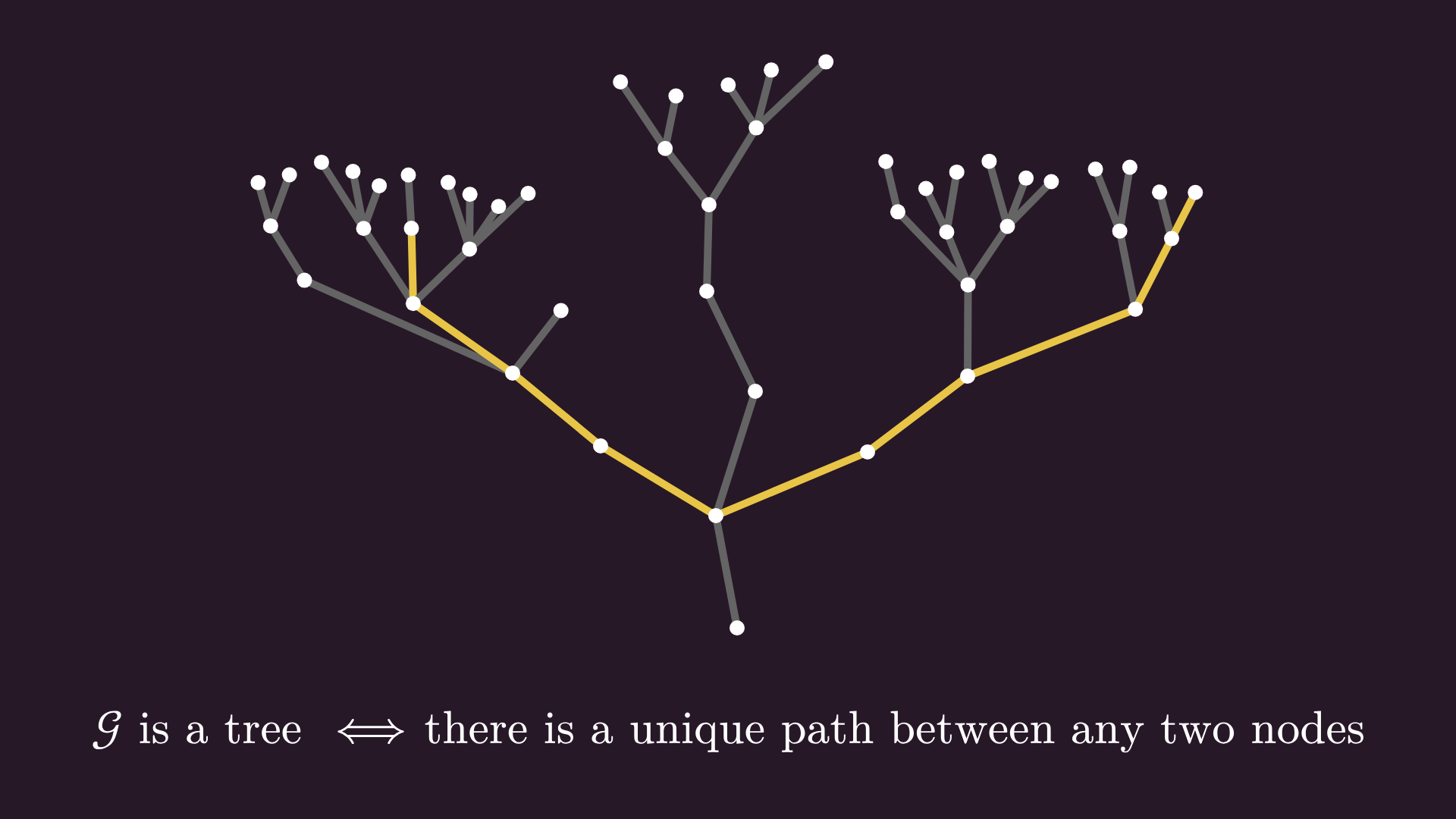
Remember my comment about cycles blocking hierarchical orderings? This is what I was talking about. Without cycles, we can just pick a node that we’ll call the root, and define the levels by measuring other nodes’ distance from the root. Which we can, because there’s only one path between the root and any other node.
Oh, and you can assign the role of root to any node you want. This graph below is the same as our example above, just with a different layout.
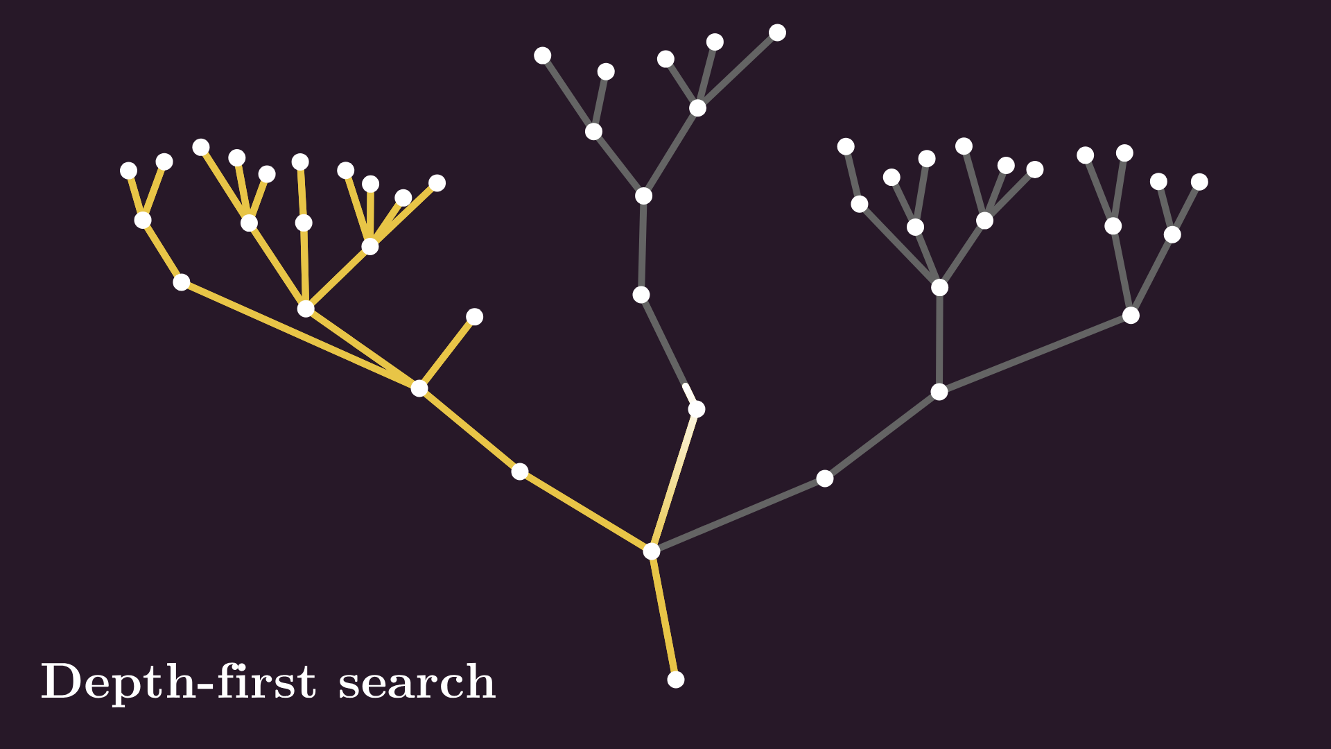
We can also beautifully illustrate search algorithms on trees. For instance, if we launch a depth-first search from the root, we can see the path going as deep as it can (hence the name depth-first), backtracking only when it runs out of depth.
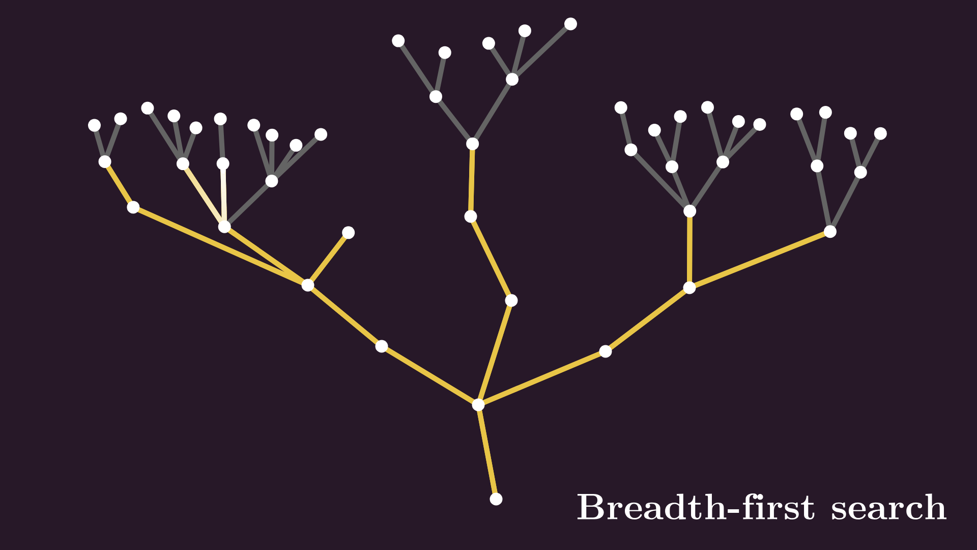
On the other hand, breadth-first search explores the graph level by level, only moving deeper when there are no more nodes left on the same layer.
Here’s a fun application of trees and search: finding our way out of labyrinths. A labyrinth can be represented by a tree graph, and we can use search algorithms to find our way out.
Launching a depth-first search is the same as following the famous “left-hand rule”: by touching the wall with our left hand and following it relentlessly, we’ll always find the exit.
One more application: decision trees. Here’s a two-dimensional dataset with two classes, and our job is to build a classifier.
The simplest way is to build a decision tree. Let me explain.
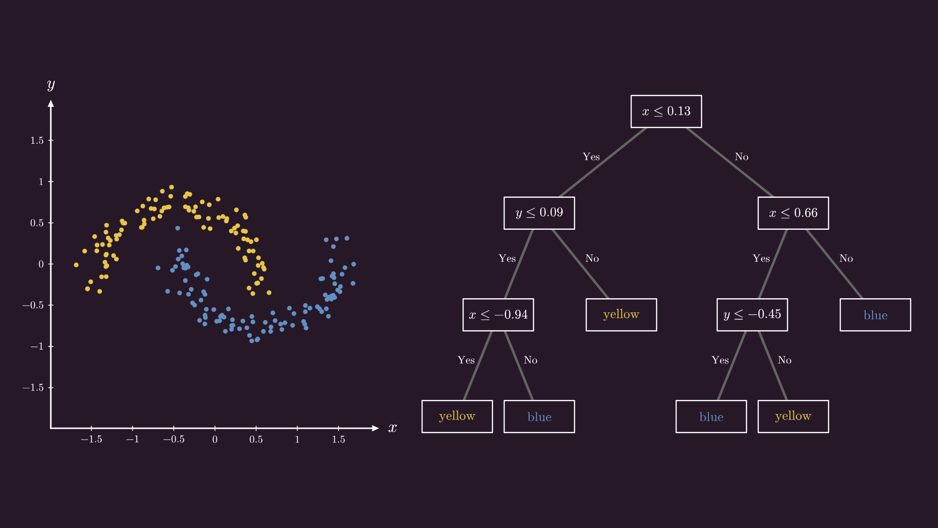
Suppose that a new sample arrives, and we want to find whether it’s blue or yellow. By asking a couple of questions, we can get an accurate prediction.
The first question in our tree: is x ≤ 0.13?
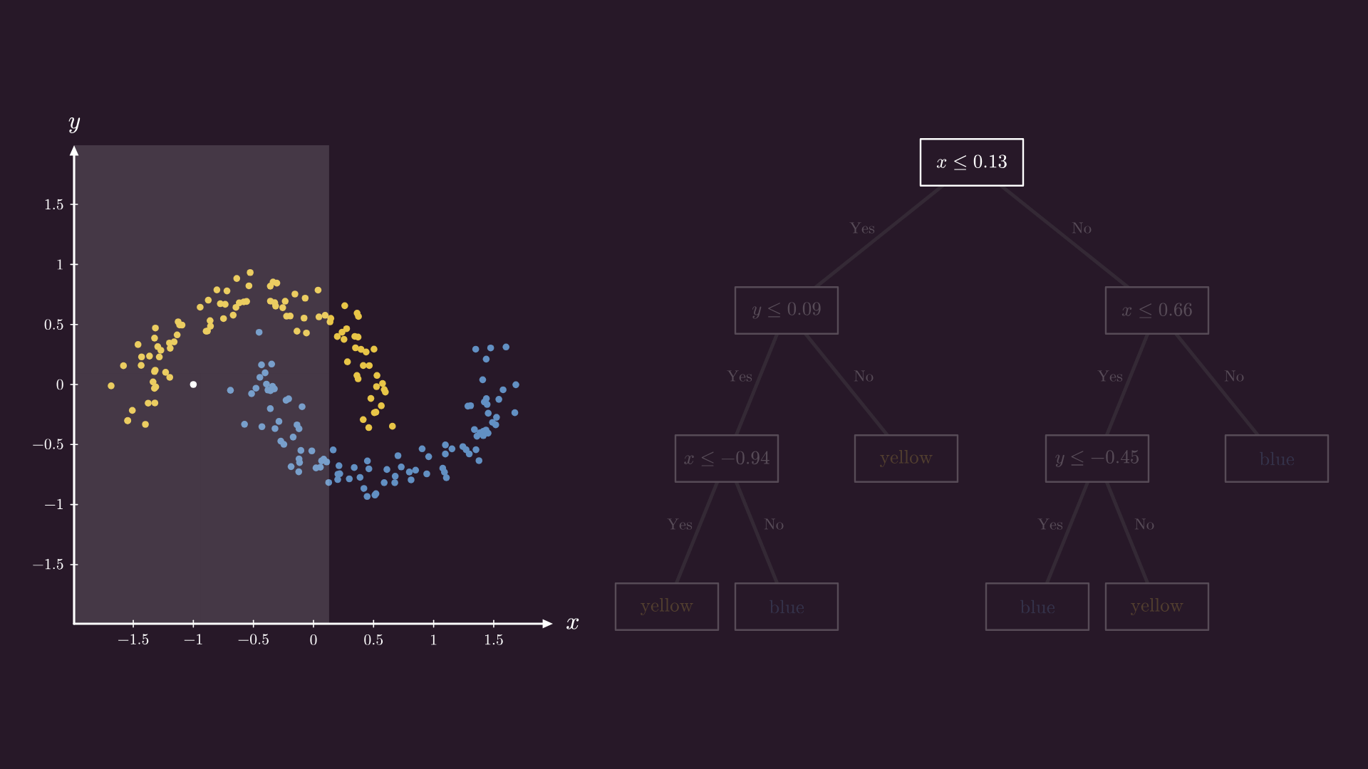
Yes, so we move towards the left. Is y ≤ 0.09?
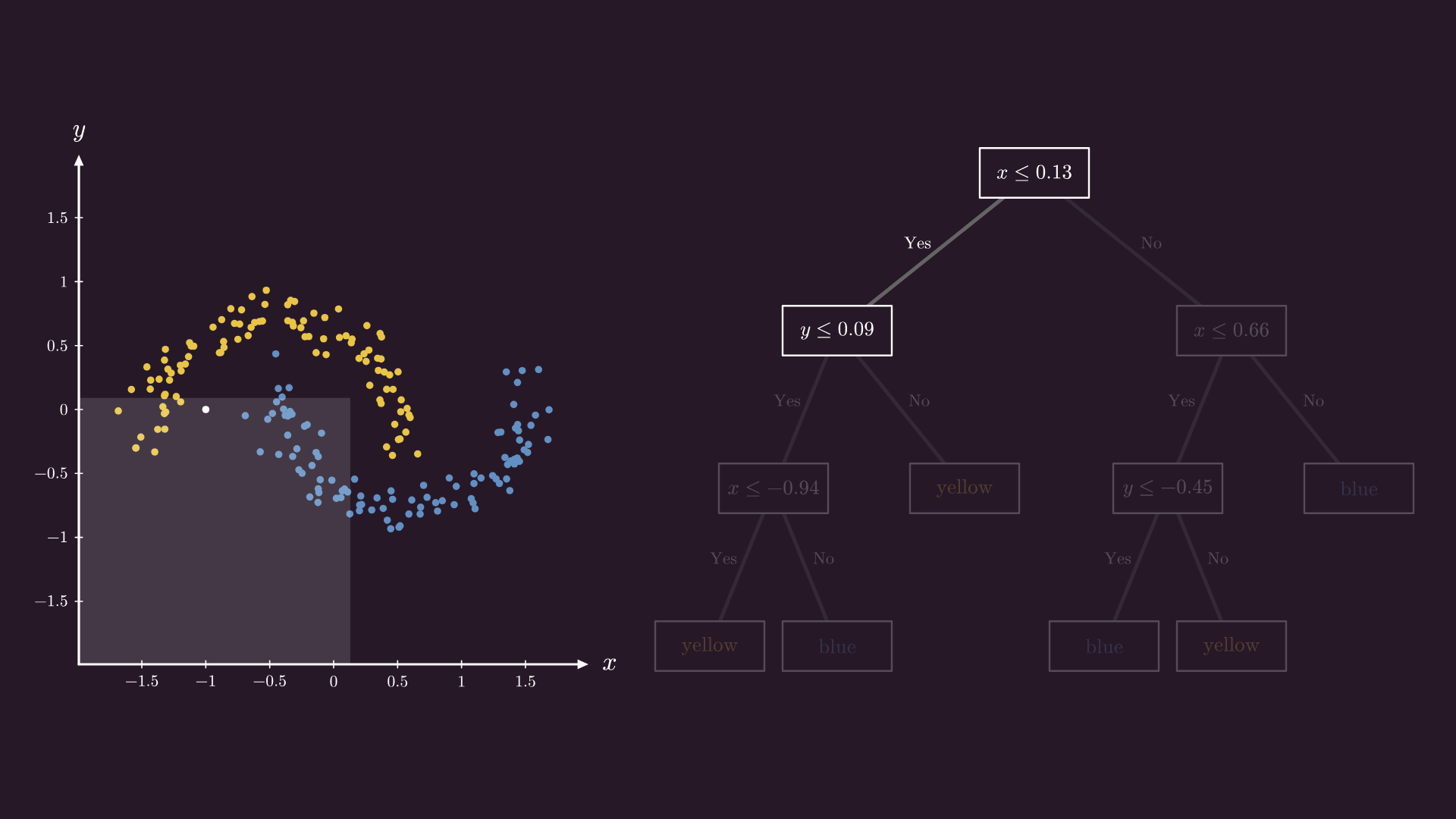
Yes once more, so we can go another level deeper. The final question: is x ≤ -0.94? Yes for the third time, and we arrive at the decision: the new point is predicted to be yellow.
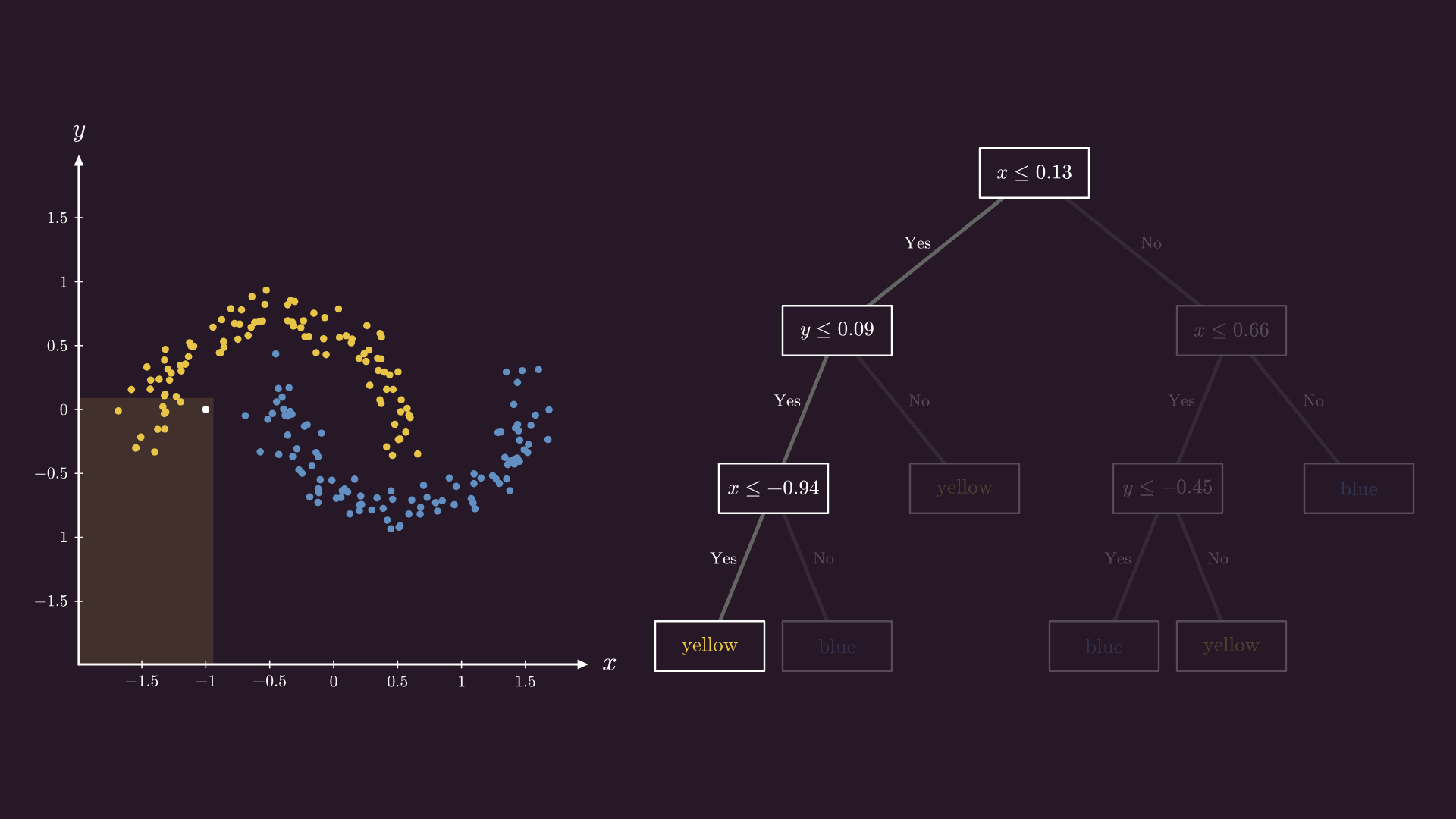
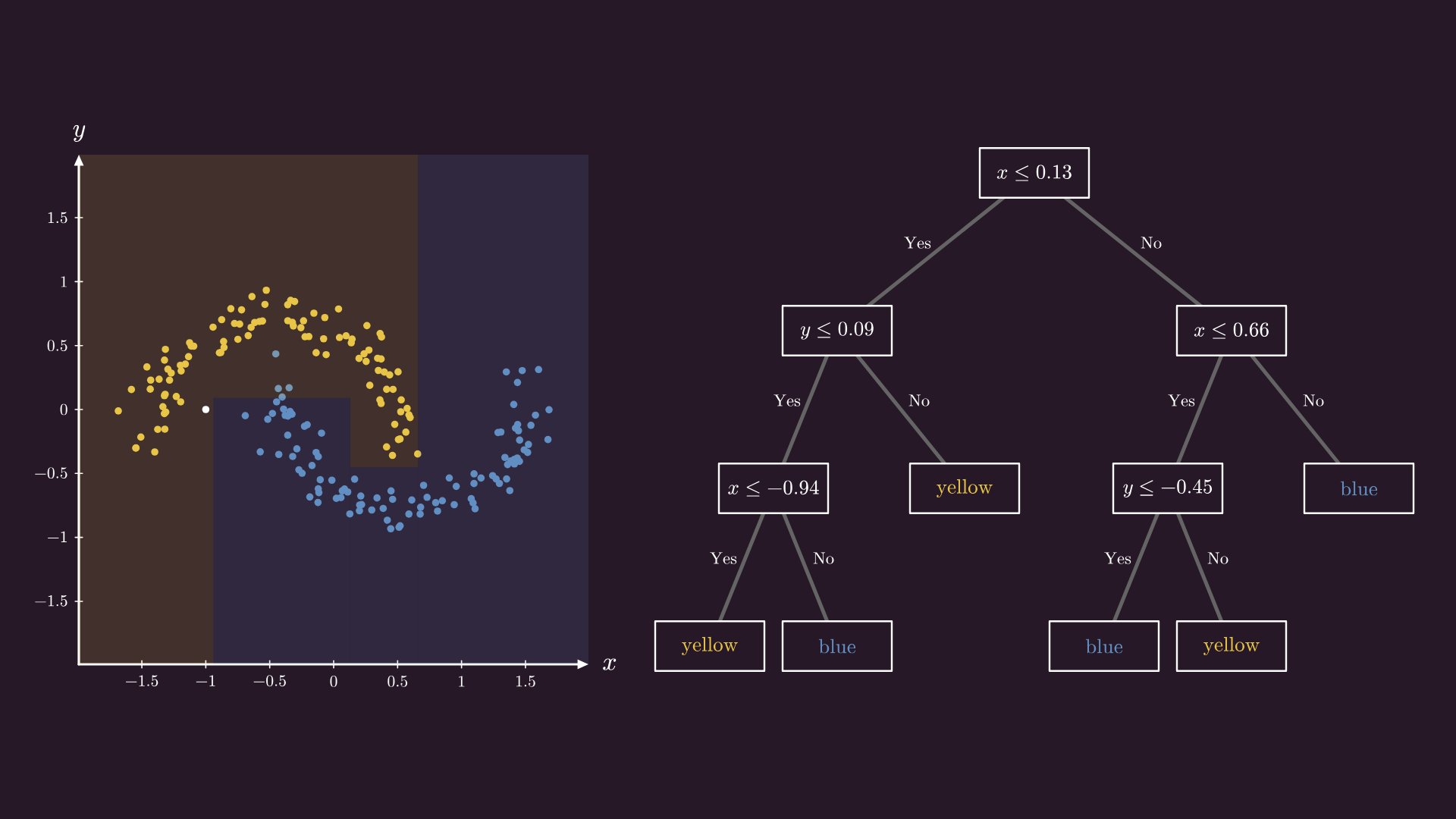
Decision trees split the feature space into rectangular regions. They are easy to navigate, lightning fast, and surprisingly accurate. On tabular data, they are state-of-the-art algorithms, winning Kaggle competitions left and right.
Hamiltonian paths and cycles
Alright, let’s move forward. I have praised trees so much that you would think that they are the best thing since the discovery of the wheel, but they have undesired properties as well.
For instance, if you think of this tree as the road network between cities, and you have to visit them all, you would waste a lot of fuel by having to go back and forth, traversing edges repeatedly.
However, road networks are definitely not trees: the web of highways is full of paths and cycles, allowing us to travel efficiently instead of forcing us to travel on the unique path. Among those paths and cycles, those that touch each node exactly once are special; we call these Hamiltonian.
These are not guaranteed to exist, but in this graph below, we have both: a Hamiltonian path:
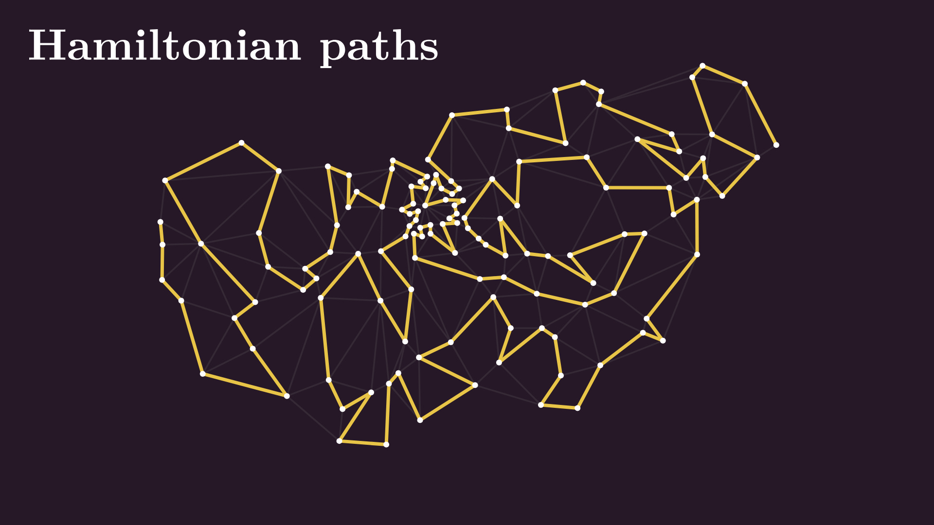
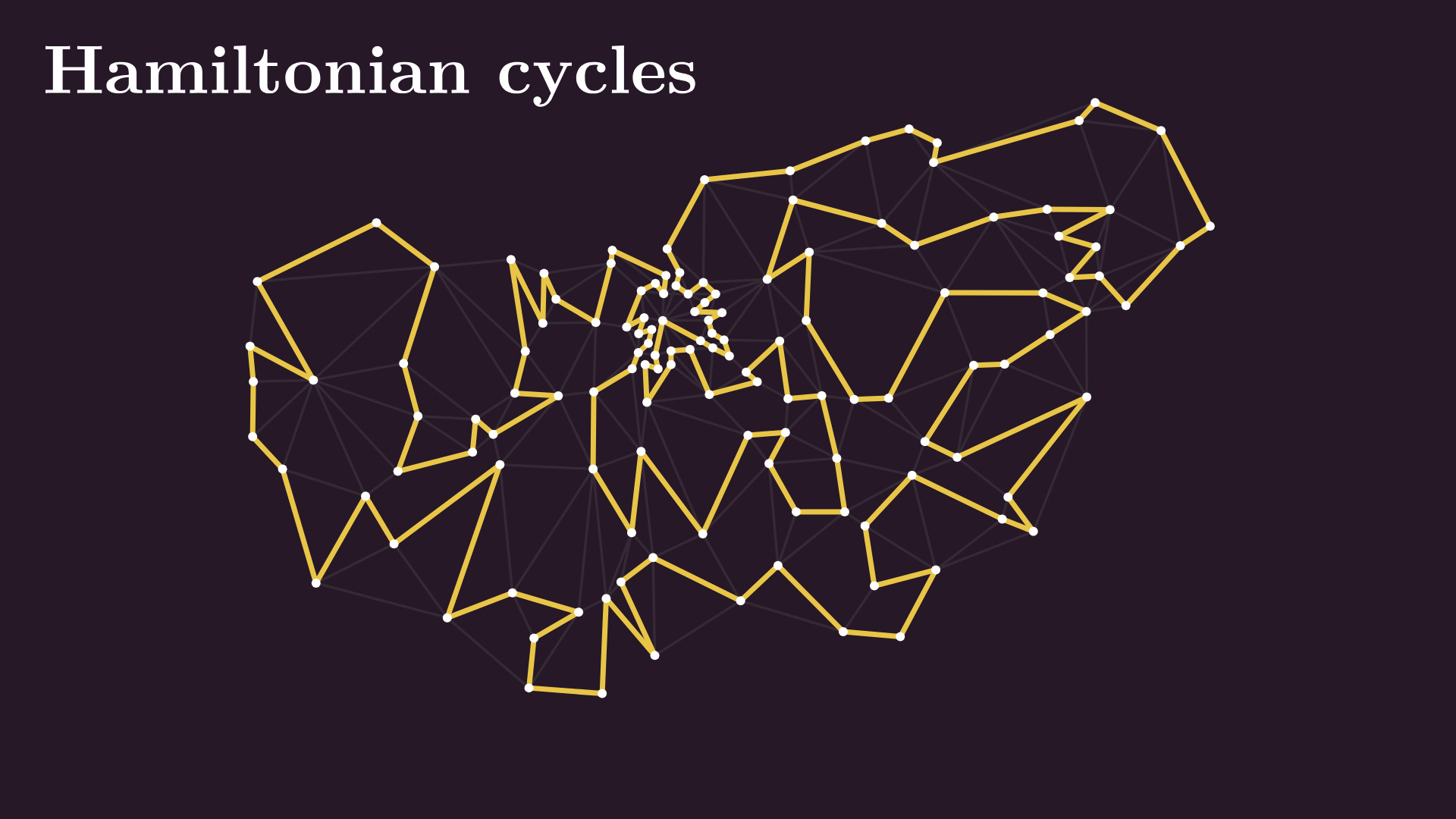
…and a Hamiltonian cycle. Finding them is a computationally complex task with immense practical and theoretical applications.
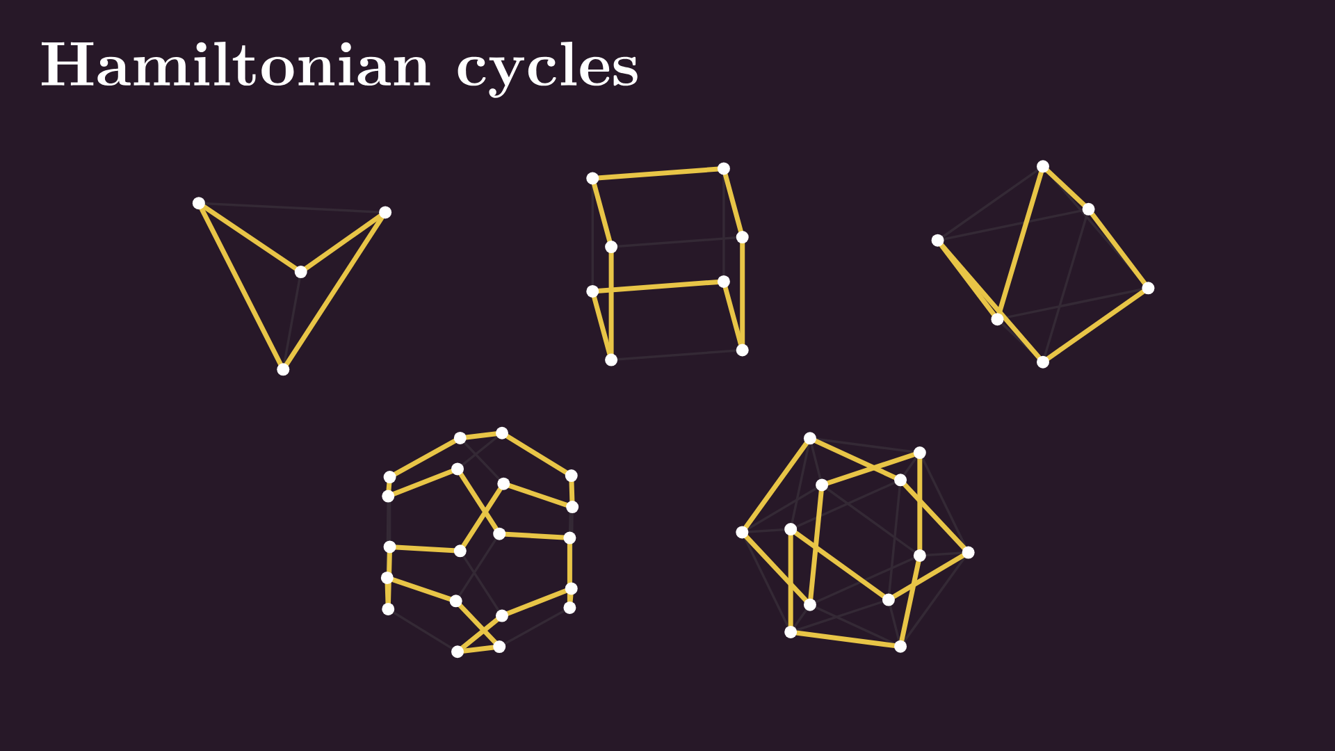
Fun fact: the edge graphs of all Platonic solids have Hamiltonian cycles as well. There are five of them, and you can traverse their nodes along the edges without repeating a single step.
Besides pathfinding, Hamiltonian paths play an essential role in assembling genomes. When a genome sequencer reads the DNA sequence, it doesn’t simply read the whole thing from start to finish. First, identical copies of full DNA strands are randomly broken into smaller pieces, which are then individually read. (BTW, this is called “shotgun sequencing”, which is one of the coolest names in science.) So, we build a graph where nodes correspond to fragments.
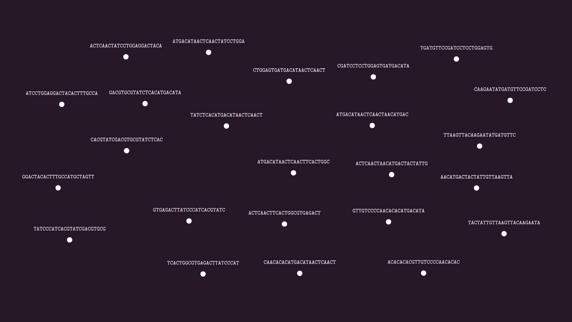
To assemble these into the full genome, we look for overlaps: if the end of a fragment overlaps with the start of another, we draw an edge from the first to the second. (Granted, we haven’t talked about directed graphs, but bear with me for a moment.)
How to assemble the full genome from the fragments? You guessed right: finding Hamiltonian paths. When such a path is available, we can just stitch the fragments along the path, obtaining a candidate for the resolution.
Planar graphs
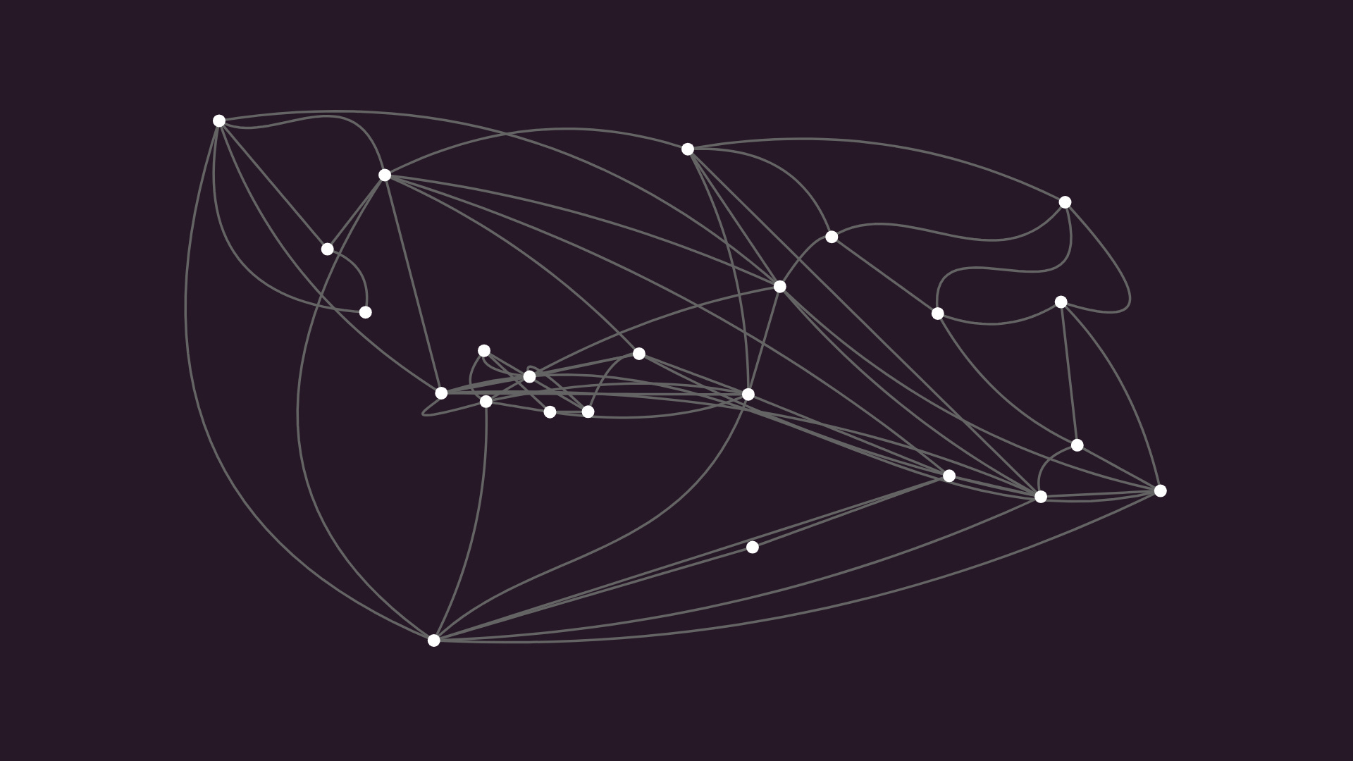
Alright, let’s change the subject and talk about a less serious topic: planar graphs. If you look at this overlap graph, you can quickly get visually overwhelmed due to the bunch of edge crossings that are present. Can we find a drawing that is without crossed edges? It turns out that no matter how we move the nodes around, and how cleverly we curve the edges, we cannot untangle this specific graph.
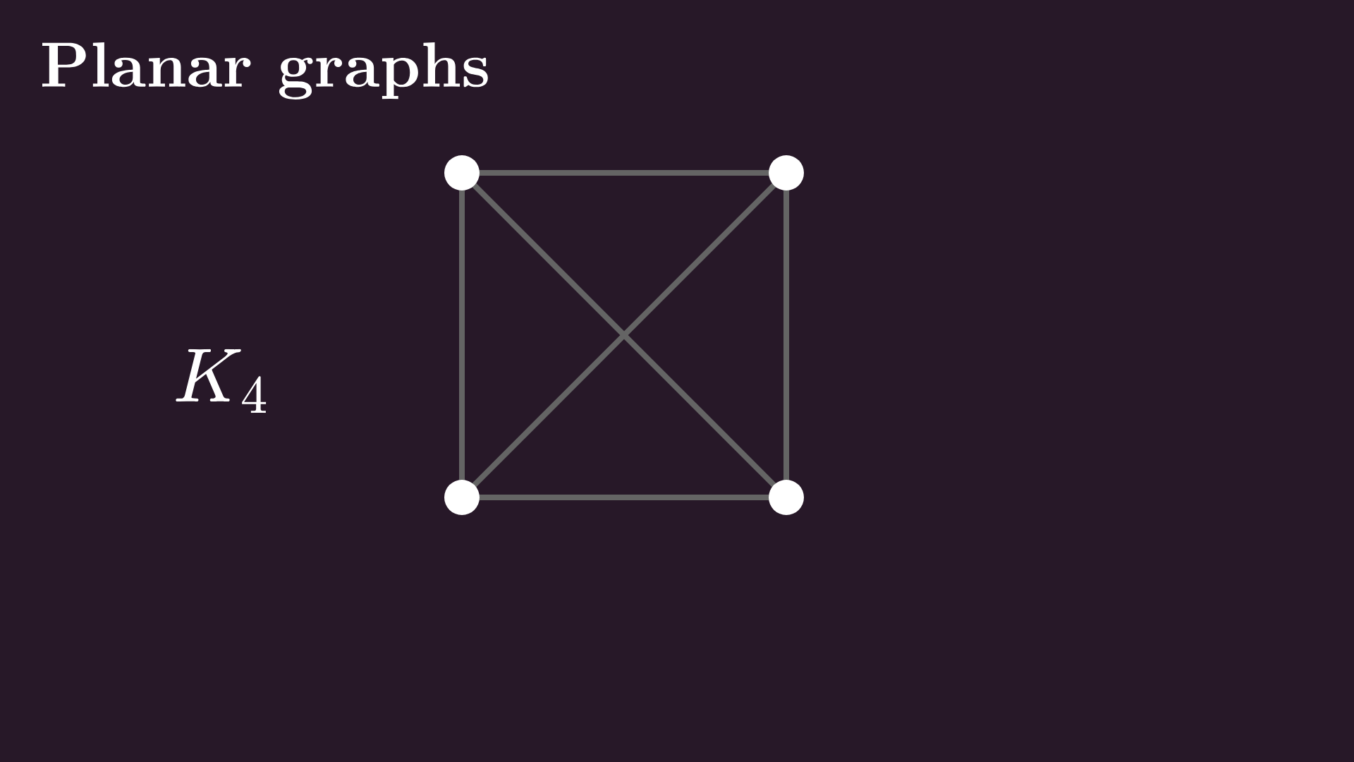
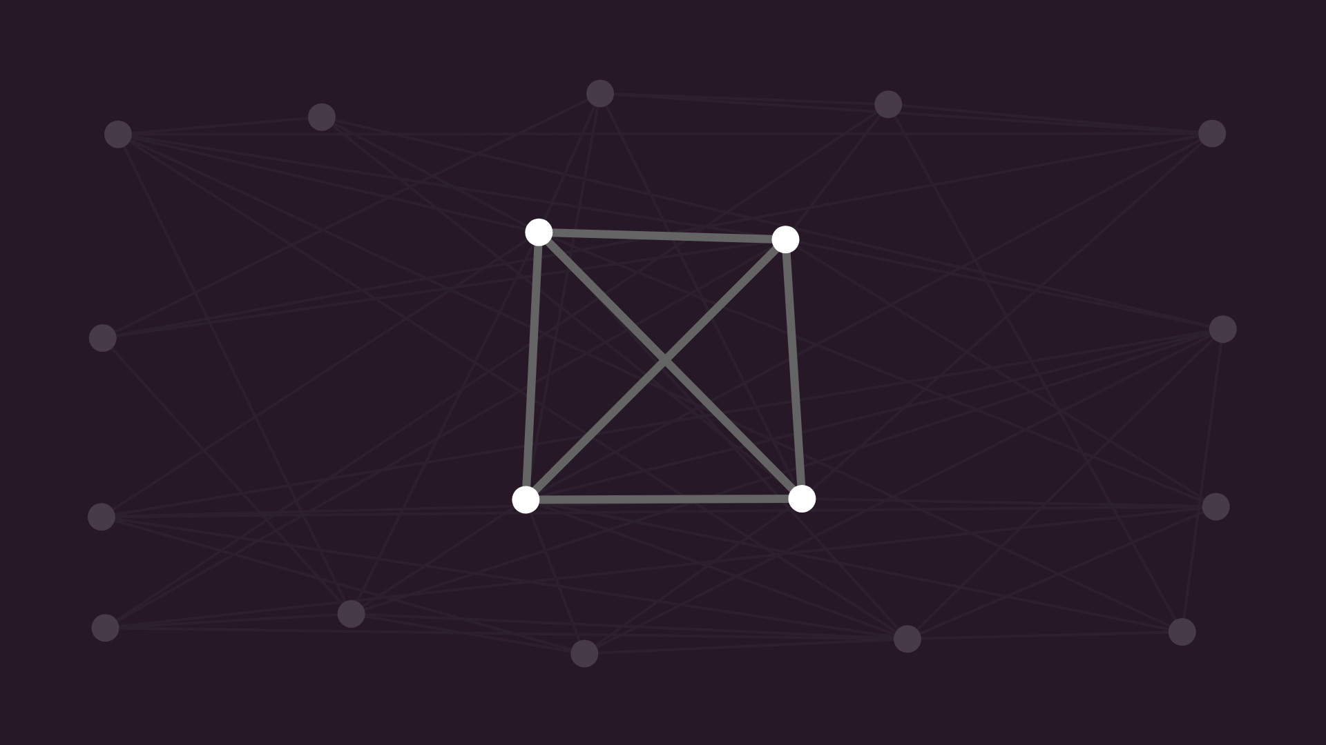
We’ll see why, but let’s start at the beginning. We say that the graph is planar if we can draw it without any edges crossing. For instance, the complete graph of four vertices, otherwise known as K₄, is planar.
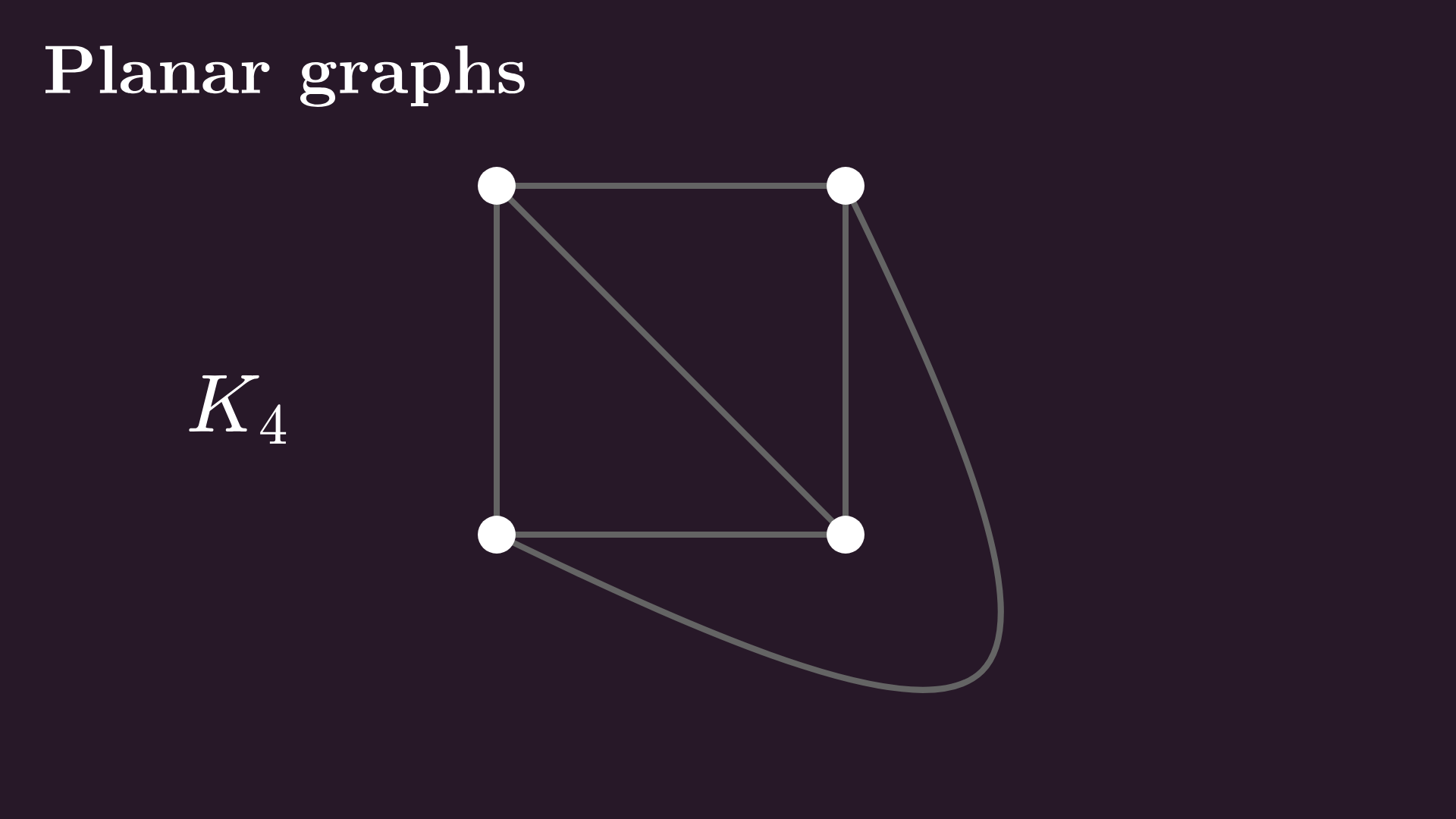
We can show the planarity by finding a drawing without crossed edges, like curving a crossing edge, or moving one node inside. See, I told you not to confuse a graph with its drawing.
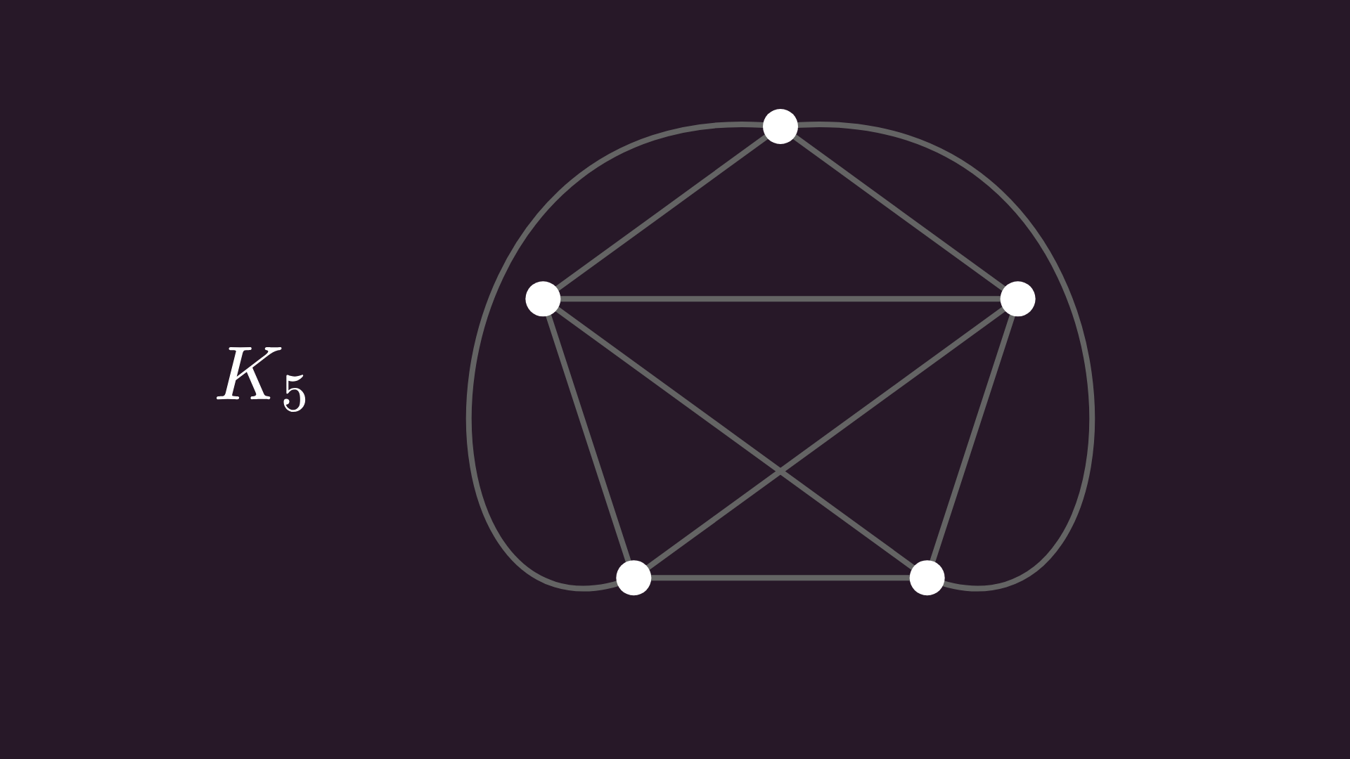
Let’s add one more node and complete the graph. Is K₅ a planar graph?
Surprisingly, no matter how hard you try, it’s impossible to untangle K₅.
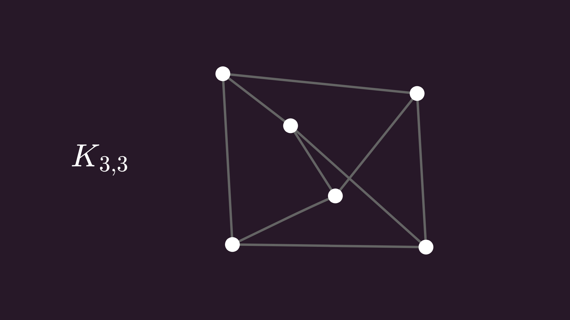
We’ll soon see why, but first, another nonplanar example: the complete bipartite graph of 3 and 3 nodes. This is known as the “utility graph”, but in Hungary, where I went to school, we just call it the 3-houses-3-wells graph.
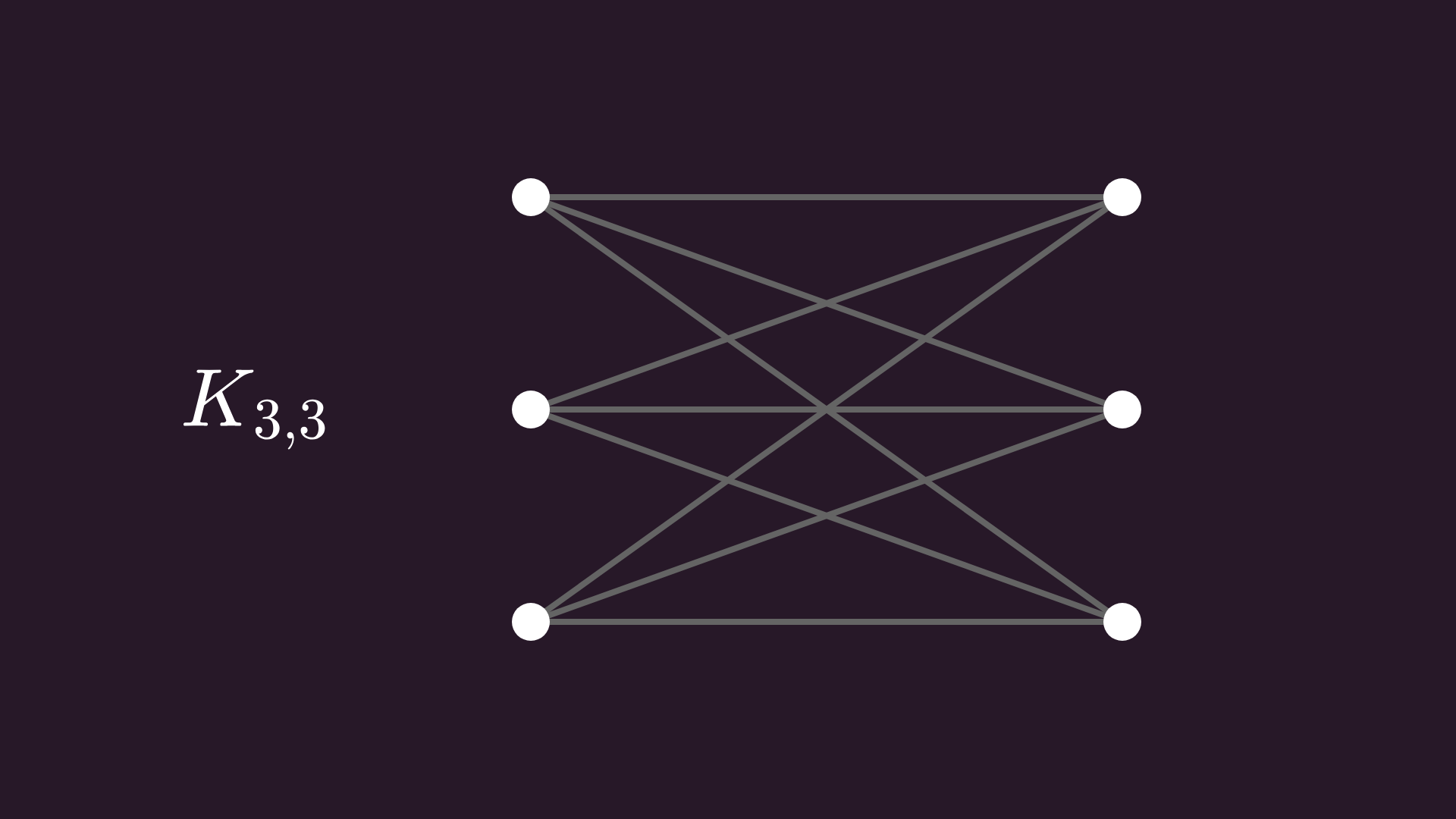
As before, no matter how hard you try, you can’t untangle all the crossings. But how can you be so sure that just because you cannot find a planar drawing, it doesn’t exist?
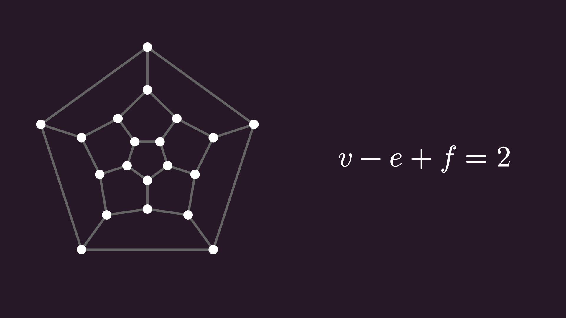
To prove this, let’s see another example. As it turns out, the edge graph of every convex polyhedron is planar. For instance, here’s the graph of the dodecahedron, one that we saw a couple of times previously.
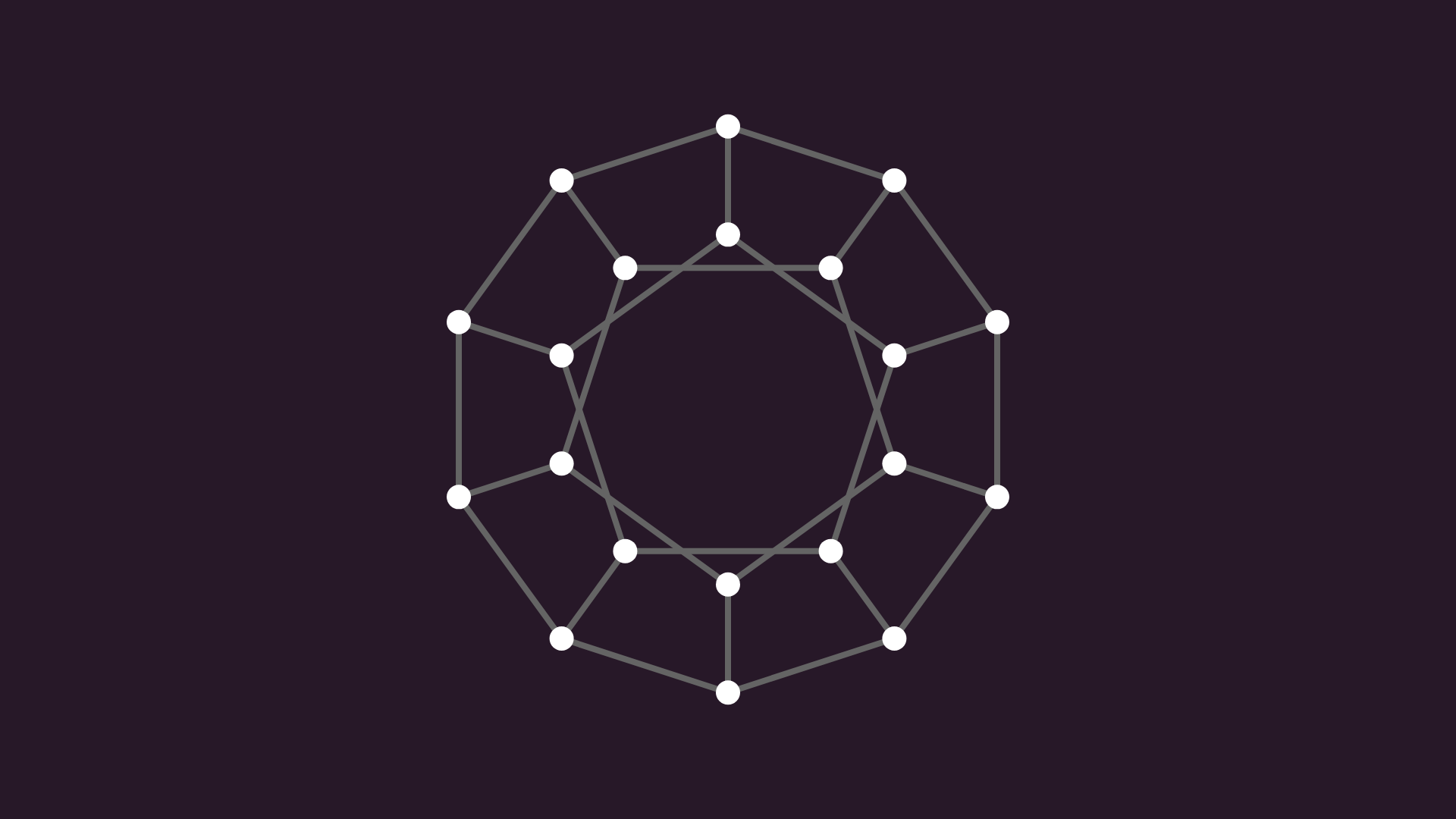
We can find a planar layout by picking a face, and laying the graph around it, like you are seeing right now.
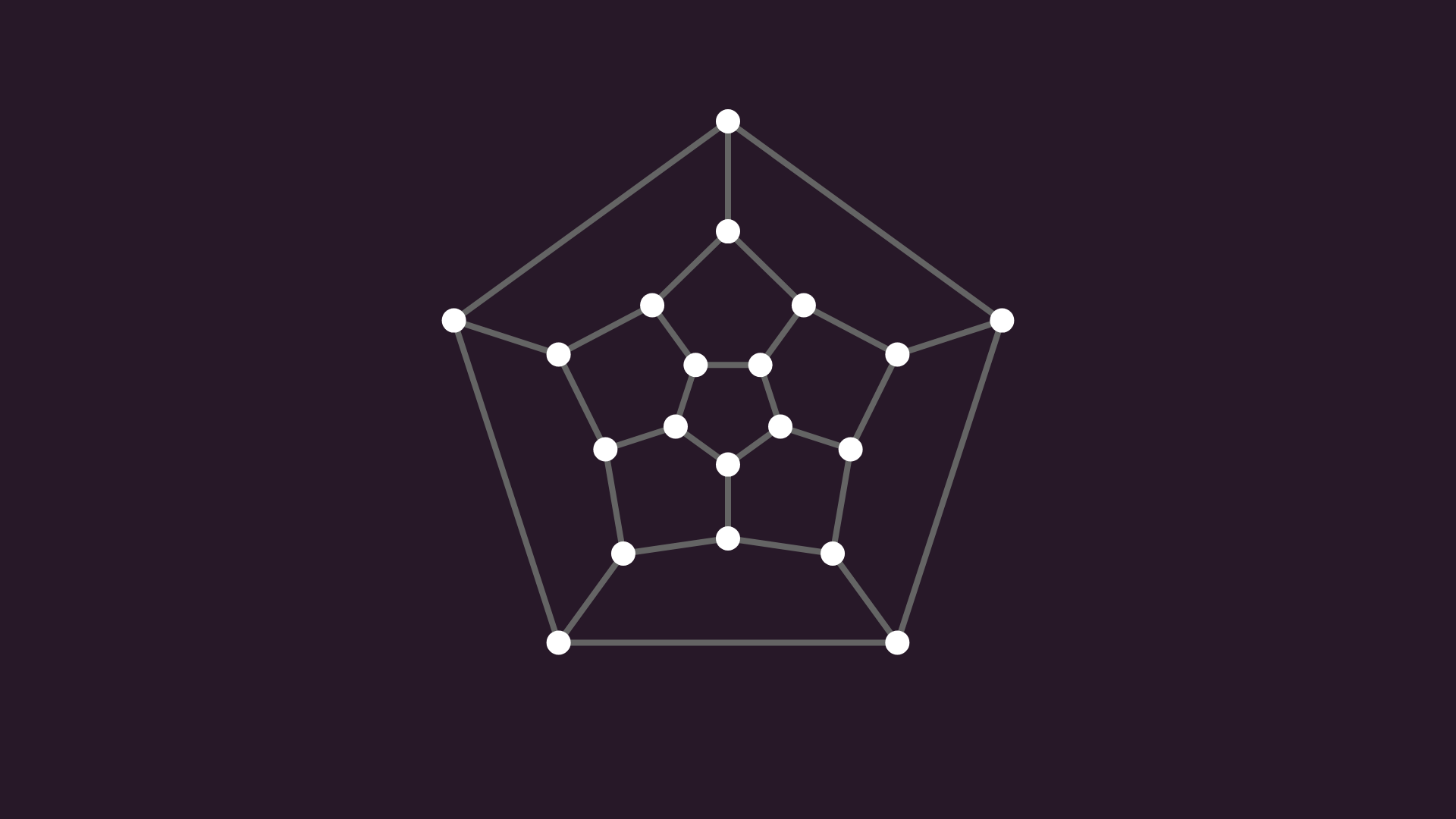
Now, let’s denote the number of nodes by v, the number of edges by e, and the number of faces — that is, the regions bounded by edges — by f. As it turns out, v - e + f always equals 2 for connected planar graphs, or in other words, v - e + f is an invariant. This is called Euler’s formula, one of many formulas named after Euler.
Besides Euler’s formula, we can make another observation for planar graphs: as each edge borders two faces, and each face is bordered by at least three edges, summing it up for all faces (and noticing that we counted each edge twice), we obtain that 2e is greater than or equal to 3f. Substituting Euler’s formula into this new inequality, we obtain that 3v - 6 is greater than or equal to e.
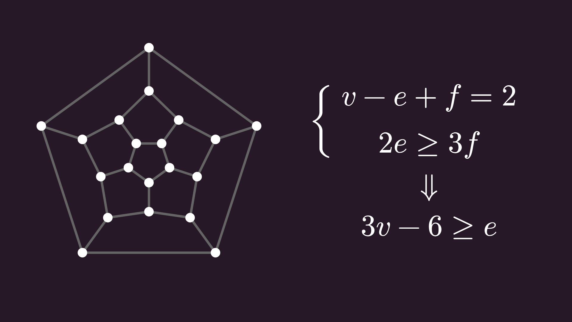
Why are we talking about this? Remember K₅, a graph we’ve seen earlier? I told you that it’s not planar, but we haven’t seen a proof, only a couple of failed attempts at finding a drawing without edge crossings. Now, K₅ has five nodes and ten edges; thus 3v - 6 equals 9, so our inequality is not satisfied; hence K₅ cannot be planar. There’s a similar proof for K₃,₃, which I’ll leave up to you.
One last concept before the punchline. K₅ is not planar, and we can manufacture more non-planar examples by splitting up any of the edges with new nodes. This is called a subdivision, and it’s easy to see that if the starting graph is not planar, then its subdivision is not planar either.
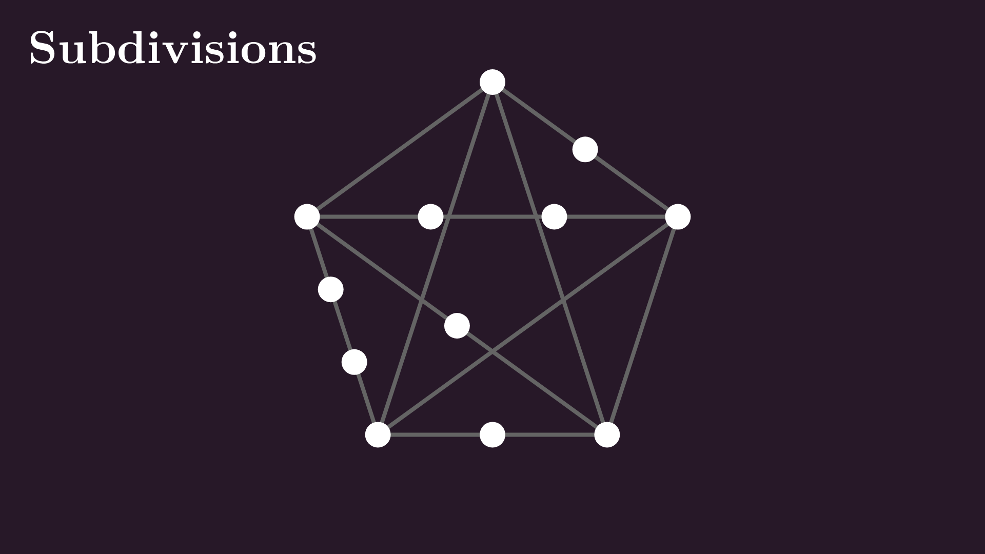
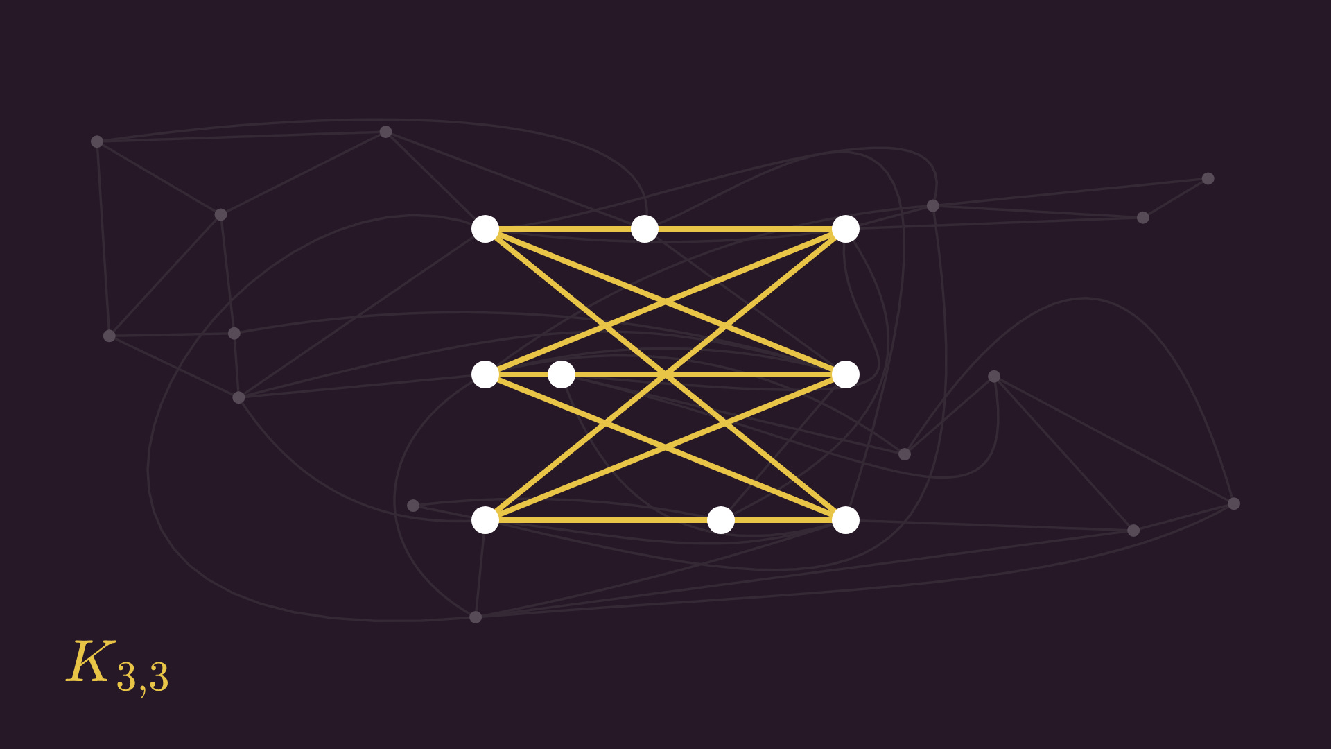
Now comes the surprise. Sure, K₅ and K₃,₃ are non-planar, but here’s the kicker: a graph is non-planar if and only if you can find the subdivision of either K₅ or K₃,₃ as a subgraph. For instance, here’s the subdivision of K₃,₃ in our shotgun sequencing overlap graph, blocking the planar embedding. This is Kuratowski’s theorem.
In a sense, K₅ and K₃,₃ are the only two unique non-planar subgraphs; we can obtain all the rest by subdividing them and adding new nodes and edges.
Vertex colorings
Alright, now let’s talk about colorings, a topic that is connected to planar graphs via one of the most famous results in graph theory. Here’s the map of Europe, and we want to color the countries.
What is the smallest color palette that we can use without having to use the same color for two neighbors?
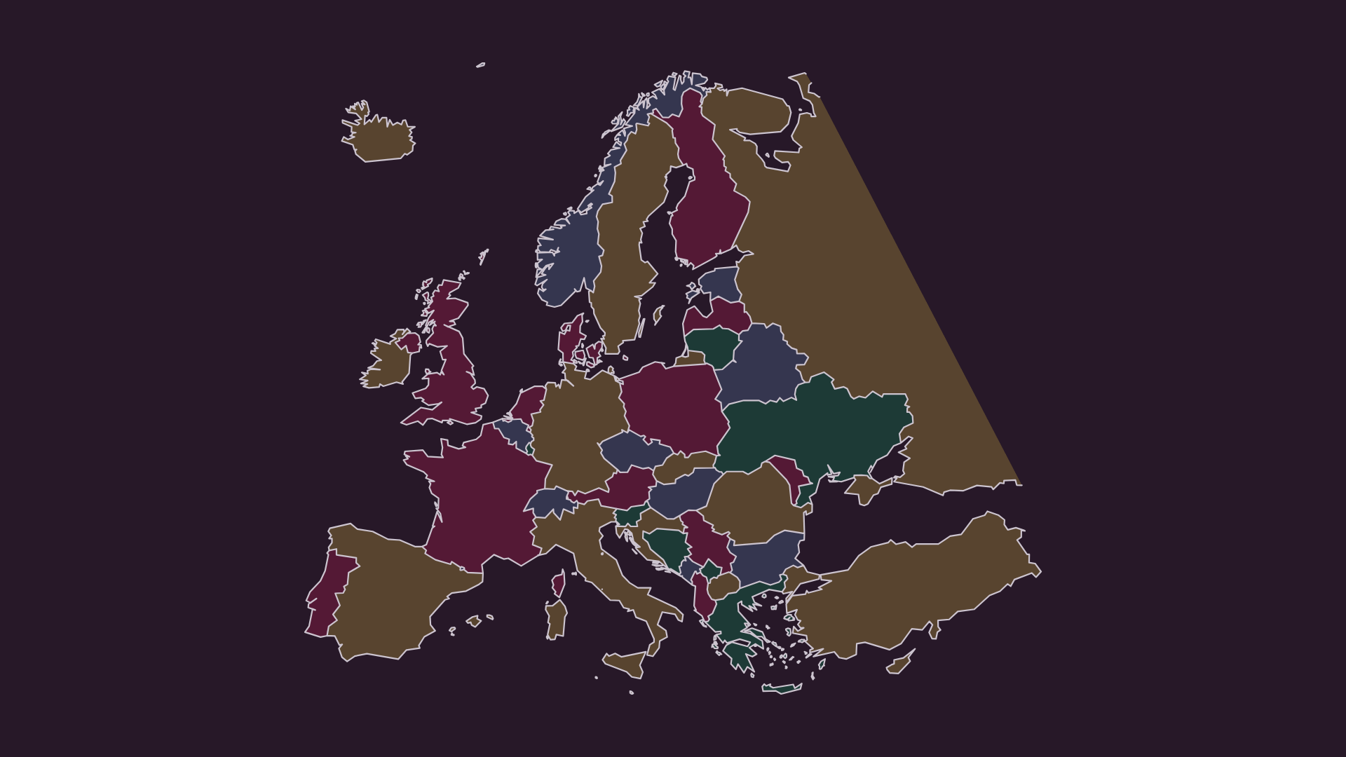
One way to translate this question to the language of graph theory is to represent each country with a node, and connect neighboring countries with an edge. This way, we are looking to color the nodes such that no neighbors share the same color.
If we want to be really academic about it, a coloring of a graph is a function that maps the vertices to a color palette, but we can think about it as an actual coloring of nodes, hence the name.
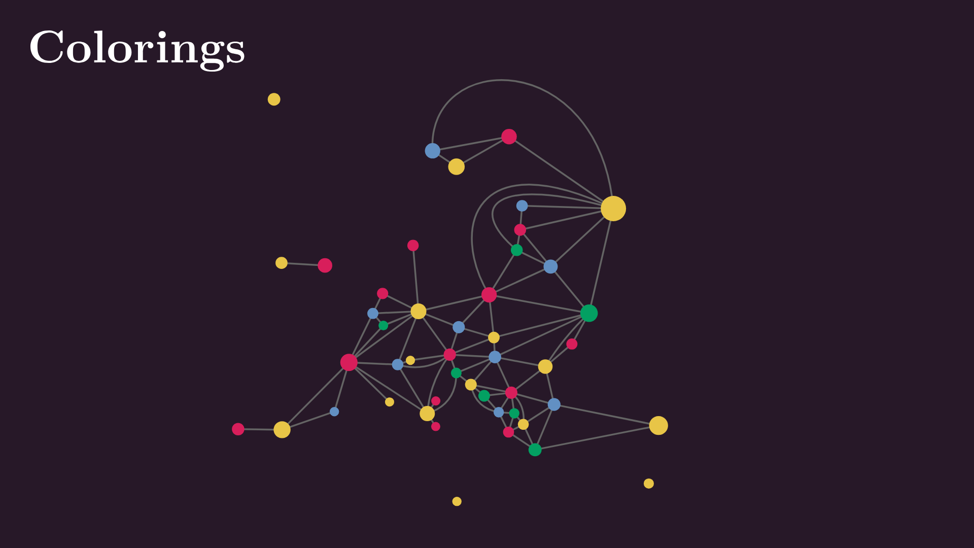
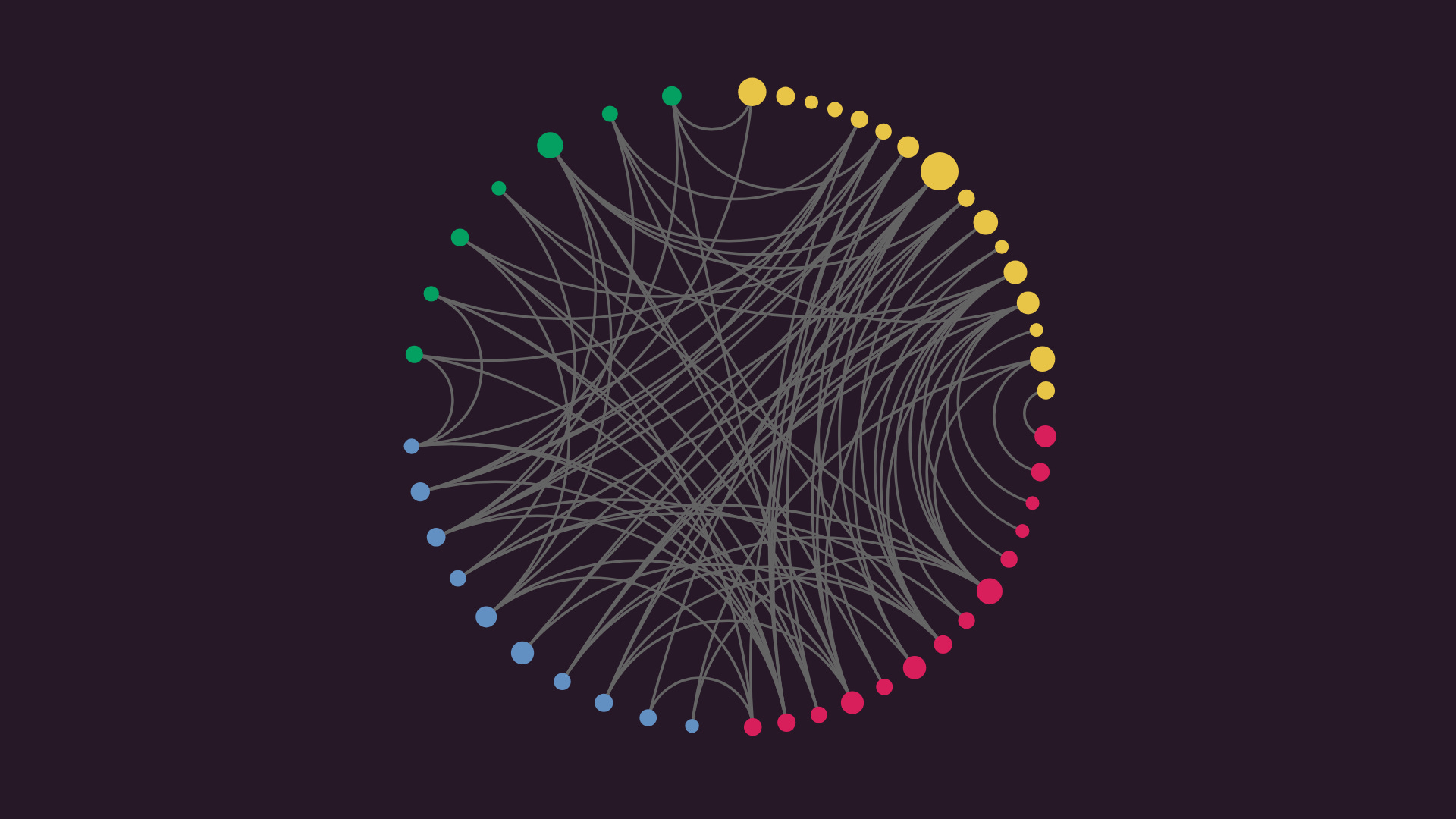
A coloring is proper when no neighboring nodes share the same color. Our map coloring uses four colors, which we can check by arranging each color into a cluster and verifying that there are no edges between vertices of the same color.
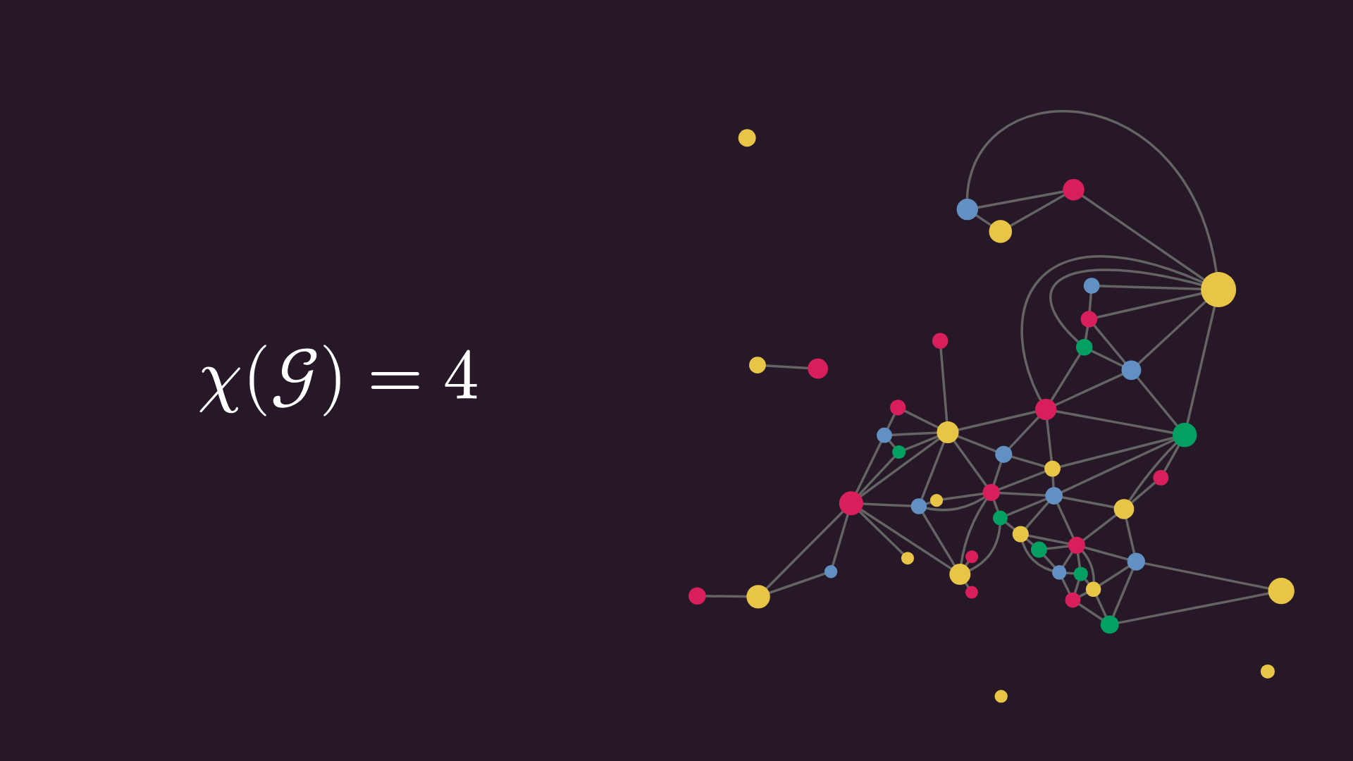
For a given graph, the minimum number of colors required for a proper coloring is called the chromatic number, denoted by the Greek letter χ.
We know that the chromatic number of this graph is less than or equal to four, because we managed to color it with four colors. But can we do it with fewer? No: Belgium, France, Germany, and Luxembourg form a four-clique, that is, four nodes that are all connected with each other.
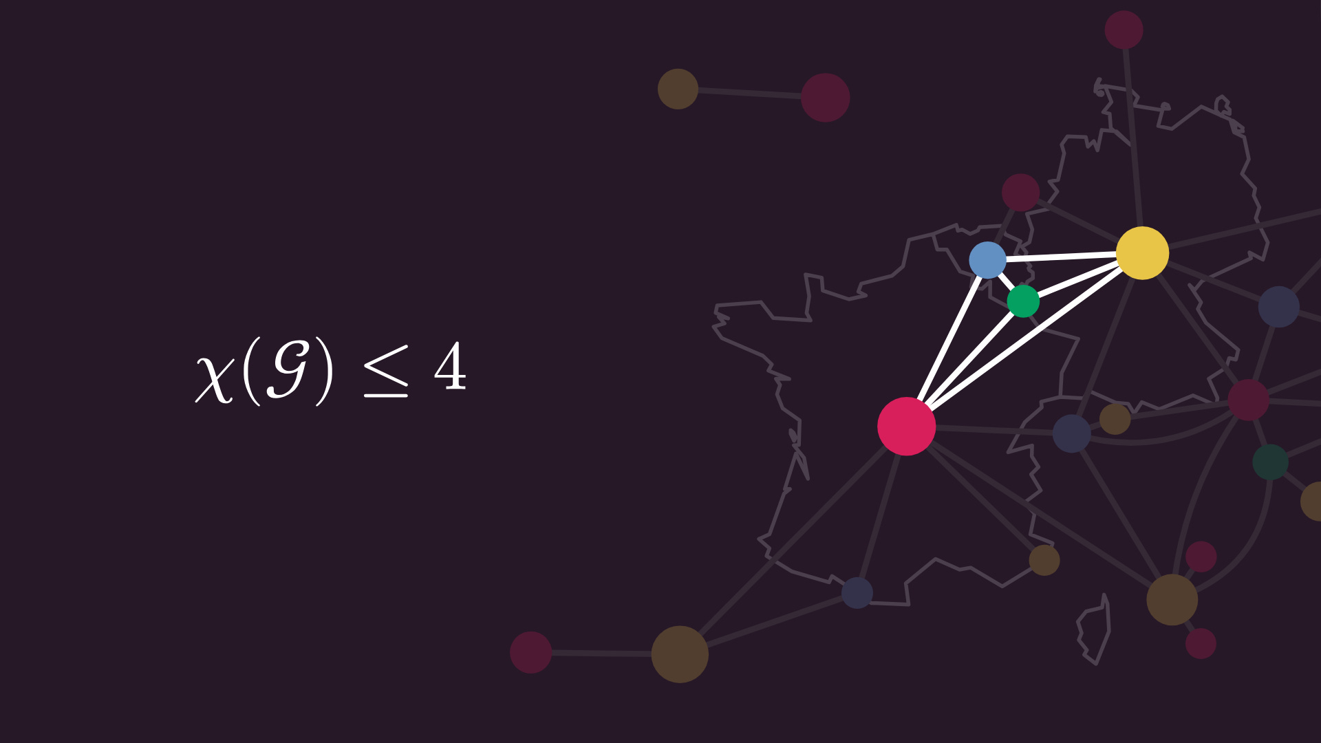
This subgraph blocks any proper colorings with fewer than four colors. So, the chromatic number is exactly four.
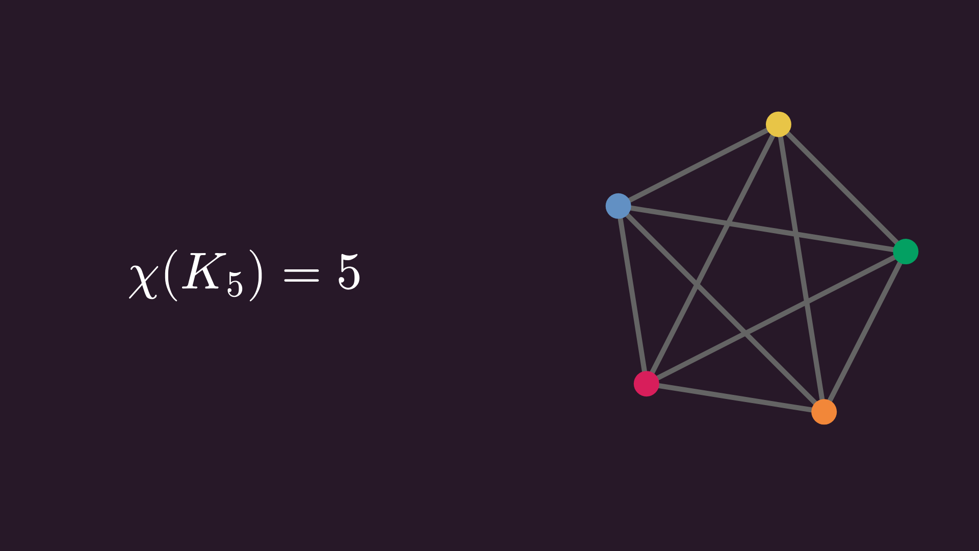
Computing the chromatic number is a notoriously hard problem. It is easy to see that the chromatic number of a complete graph is equal to the number of nodes, but a high chromatic number does not imply a complete subgraph at all. One construction that shows this produces the Mycielskian graphs, that is, triangle-free graphs with arbitrarily high chromatic number.
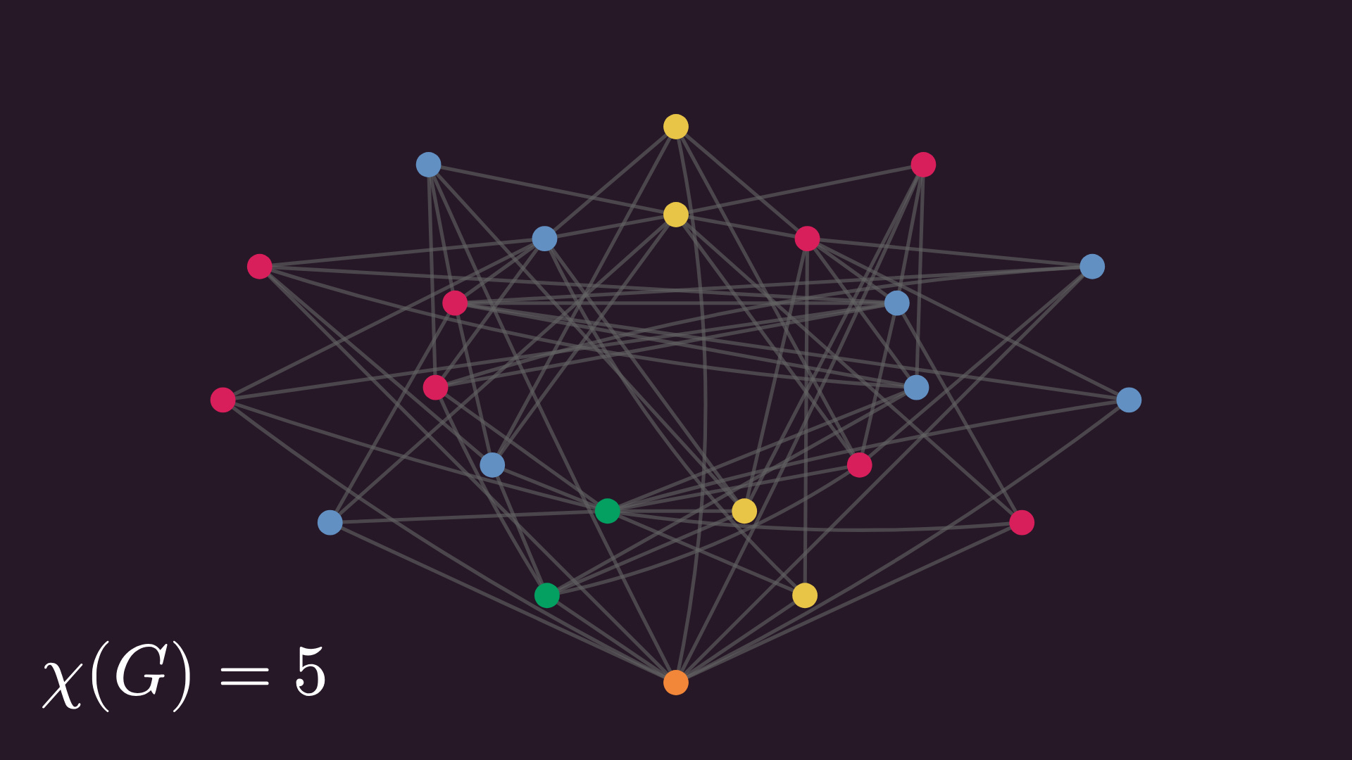
We start with a five-node cycle that requires three colors, and contains no triangles. The Mycielskian construction first lays out the nodes in order, copies each node, connects each copy to the neighbors of its corresponding original node, and adds an extra node that is connected to all the copied nodes.
Due to the construction, the copied nodes can have their originals’ color, but the extra node needs a new one to maintain a proper coloring. The graph still doesn’t include any triangles, but the chromatic number increased by one.
We can iteratively repeat this construction, bumping up the chromatic number each time. Here’s the next one, the next one, and the next one. We can go on and on forever, avoiding triangles and increasing the chromatic number with each step.
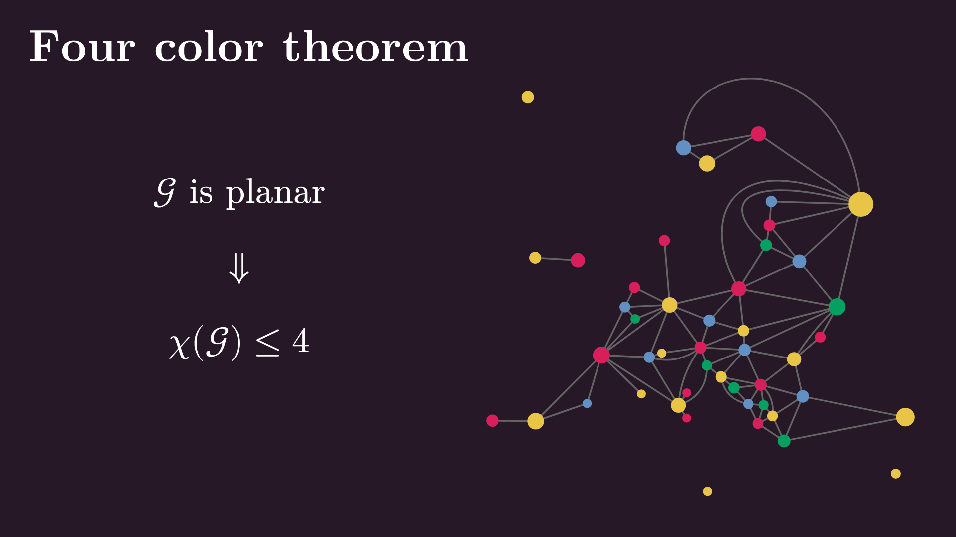
Alright, now let’s get back to where we started. How did I know in advance that the graph of Europe can be colored with only four colors? Because it’s planar, and as the famous four-color theorem states, the chromatic number of planar graphs is less than or equal to four. That’s why you can always properly color a map with four colors.
Edge colorings
Now that we’ve dipped our toes into vertex colorings, you might ask the question: can we color the edges? We can do (almost) everything in mathematics, so we definitely can. Just like for vertex colorings, an edge coloring is proper if all edges connected to a single vertex have different colors.
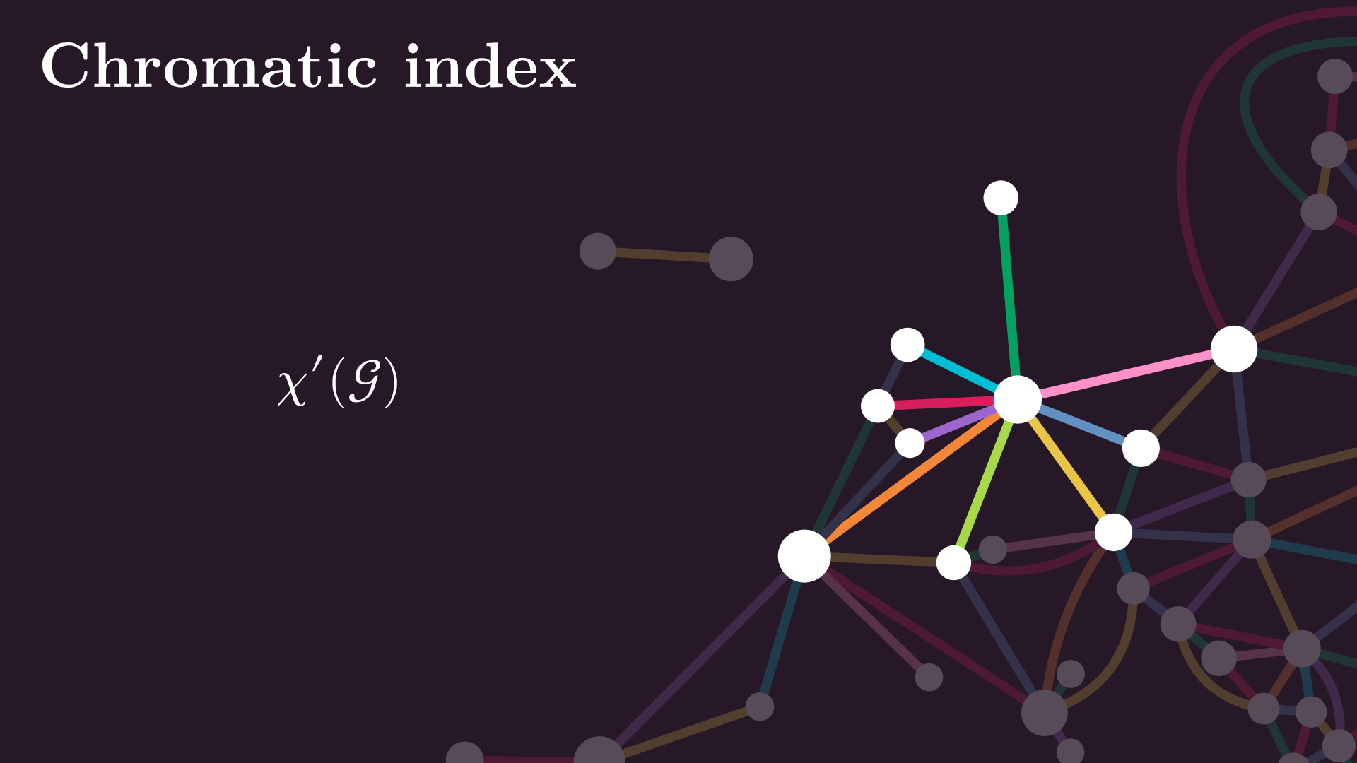
The minimal number of colors needed for a proper edge coloring is called the chromatic index, denoted by χ prime. It’s easy to see that the chromatic index is at least the maximum number of connected edges for a single node. In the graph of Europe, this is Germany with its 9 neighbors. In other words, the chromatic index is bounded below by the maximum of the degrees.
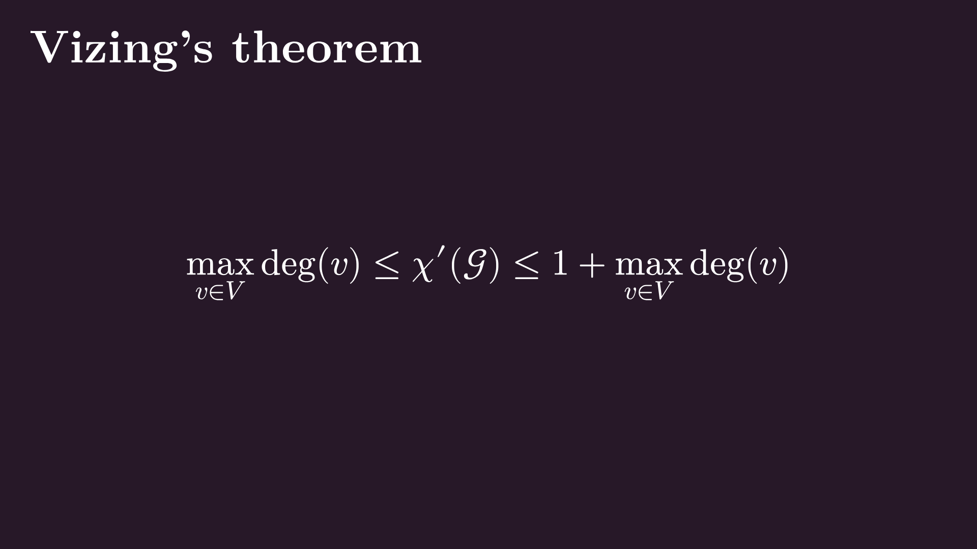
But here’s the surprising thing. The chromatic index is bounded above by the max degree plus one! This is called Vizing’s theorem, a result that limits the value of the chromatic index to two choices.
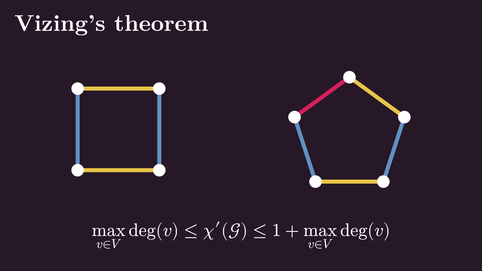
Vizing’s theorem states that there are two cases. One: the chromatic index is the maximum degree. This happens, for instance, in cycles with an even number of nodes. Two: the chromatic index is the maximum degree plus one, such as in cycles with an odd number of nodes.
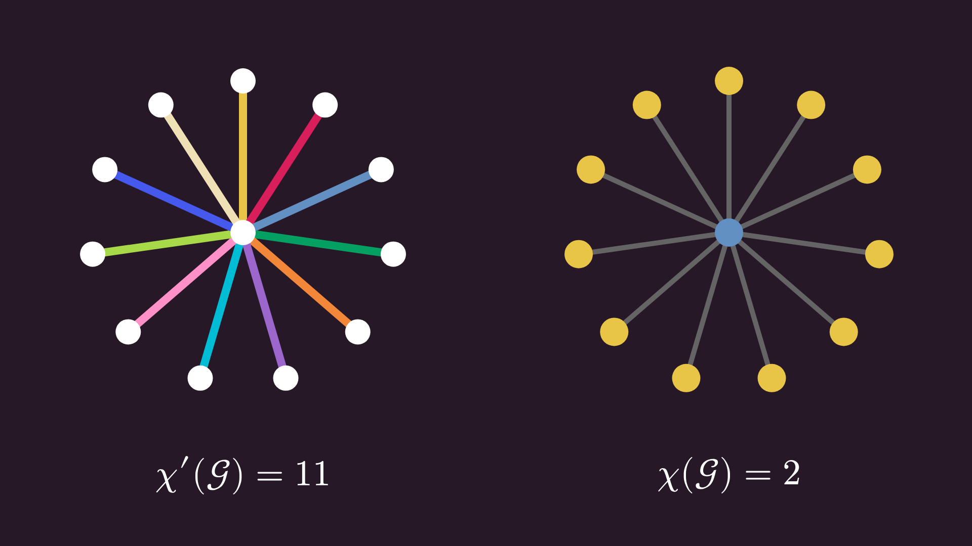
This result is in stark contrast with vertex colorings: we don’t have such a sharp lower bound there. Take a look at this star-shaped graph, with one node in the center and all other nodes attached to it. Its chromatic index is the degree of the central node, as each edge requires a unique color.
On the other hand, the vertices can be properly colored with just two colors: one for the central node, one for all the others. If we keep increasing the number of nodes connected to the central node, the chromatic index increases each time, while the chromatic number stays at two.
Ramsey theory
Now, let’s change our perspective, and instead of looking for proper colorings, let’s just use two colors; for instance, here’s such an edge coloring of K₆, the complete graph on six vertices.
Finding substructures in graphs that block one property or enable another is a common theme in graph theory. Now, I want to talk about monochromatic cliques, that is, complete subgraphs that have the same edge color. In this example, we can see that there’s a blue triangle (or, in other words, a blue K₃) in the middle of our edge-colored graph.
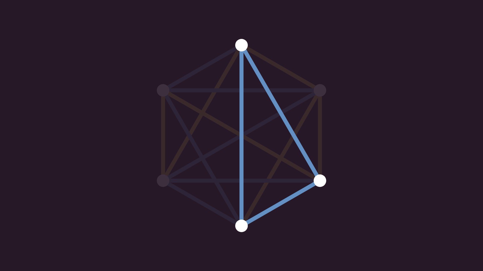
Is this an accident? No. Turns out that no matter how we color the edges of K₆, we can always find a monochromatic triangle. Instead of brute-forcing our way through all the 2^15 cases, we can use an elegant proof based on the pigeonhole principle, one of the simplest yet most powerful tools of mathematics.
Let’s start from a clean slate, and color the edges of K₆ one by one. First, we color all the edges of a single node with our two colors. Because of the pigeonhole principle, at least three of them share the same color; we’ll focus on the vertices on their other ends. If we color all the edges between them with blue, we have our monochromatic triangle. If at least one is yellow, again we have our monochromatic triangle, formed between the ends of the new yellow edge and the first node.
This is called Ramsey’s theorem, stating that if you color the edges of K₆ with two colors, you can find a monochromatic triangle, that is, K₃ as a subgraph whose edges have the same color.
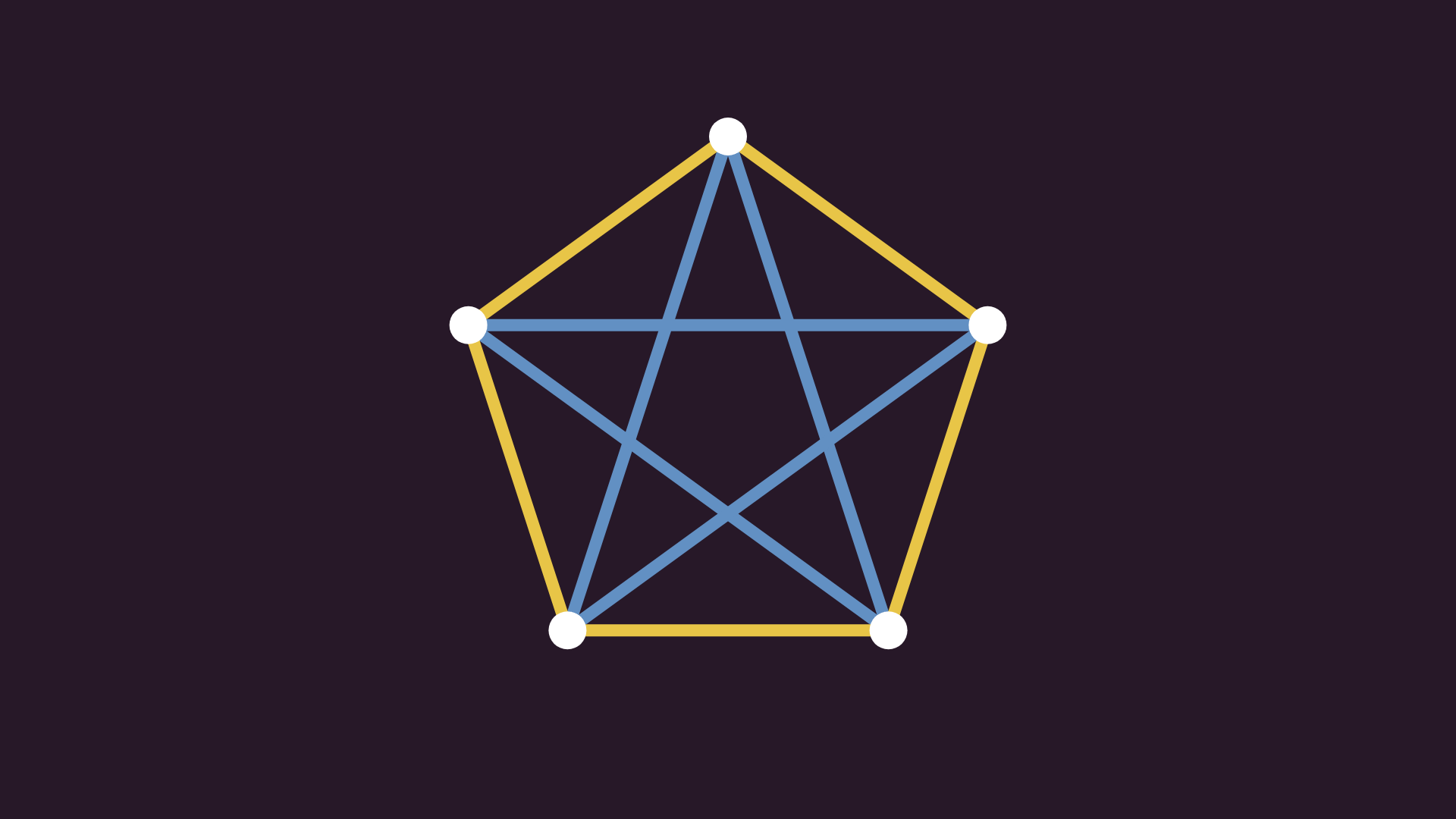
Let’s reverse the question. How large should n be to surely find a monochromatic triangle? We can instantly see that we can avoid monochromatic triangles in K₅ with this coloring, and we’ve just seen that we can’t avoid them in K₆ and above, so n is precisely six in our case.
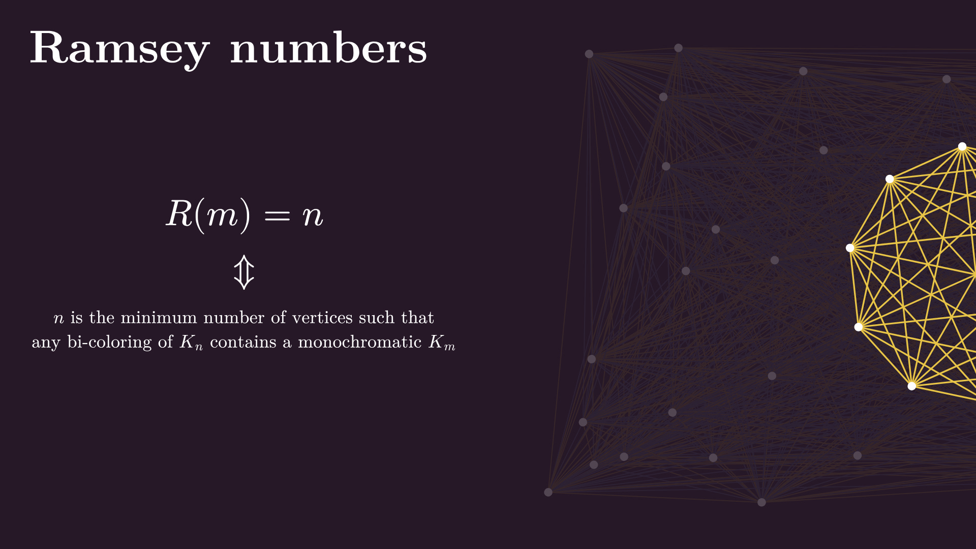
Let’s generalize even more. What if we are looking for larger regular subgraphs, like a monochromatic K₁₀? How large must our bi-colored complete graph be to guarantee such a substructure?
This question is answered by the Ramsey numbers: the m-th Ramsey number (denoted by R(m)) equals n if and only if n is the minimum number of vertices such that any bi-coloring of Kₙ contains a monochromatic Kₘ subgraph.
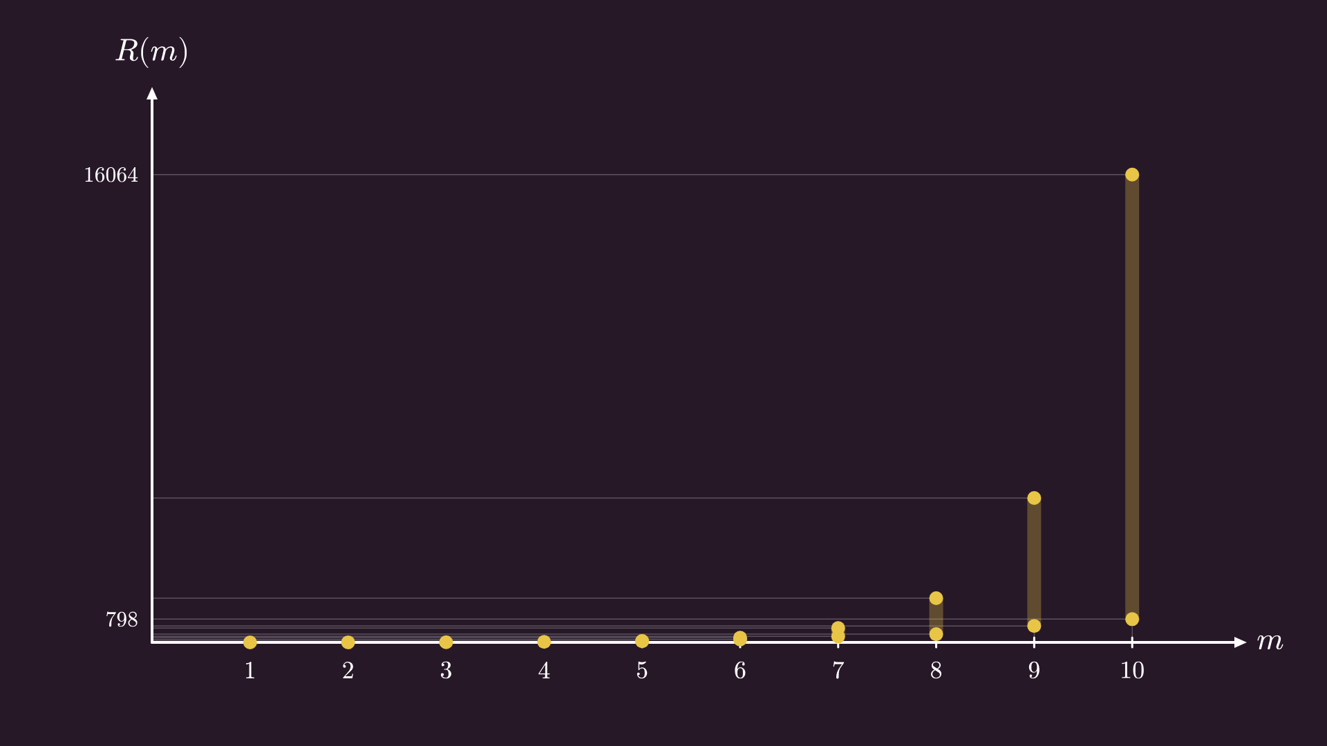
R(1) is 1, R(2) is 2, and as we’ve just seen, R(3) is 6. Now comes the interesting part. R(4) is 18, and this is the last Ramsey number we know exactly; we only know bounds for the subsequent ones. R(5) is between 43 and 46, R(6) is between 102 and 160, R(7) is between 205 and 492, and so on, as the gap between the lower and upper bounds keeps growing. As m grows, the combinatorial complexity explodes, and the Ramsey numbers become hard to find.
By the way, there’s another way to interpret Ramsey’s theorem. Instead of looking at bi-colorings of edges, simply take away the blue ones, thus obtaining a good old simple graph. R(4) = 18 says that, for example, if there is a social network of 18 people, there are 4 people who either mutually know or don’t know each other.
Weighted and directed graphs
Alright, that’s enough about Ramsey theory. Now, let’s talk about something that we’ve overlooked so far in our journey. This graph represents the “a is friends with b” relation, which is symmetric, meaning that if “a is friends with b”, then “b is friends with a” as well. If you recall the mathematical definition of graphs, this symmetry is represented by the fact that we store edges as two-element subsets of the vertices. For instance, this is how social graphs are represented by Facebook.
However, if we move on to other social media platforms, like Instagram, X, or whatever, we see that the “a follows b” relation is not symmetric! We can model this by adding directions to our edges, visually done by adding arrowheads to the edges, and mathematically done by representing edges with tuples instead. This is called a directed graph.
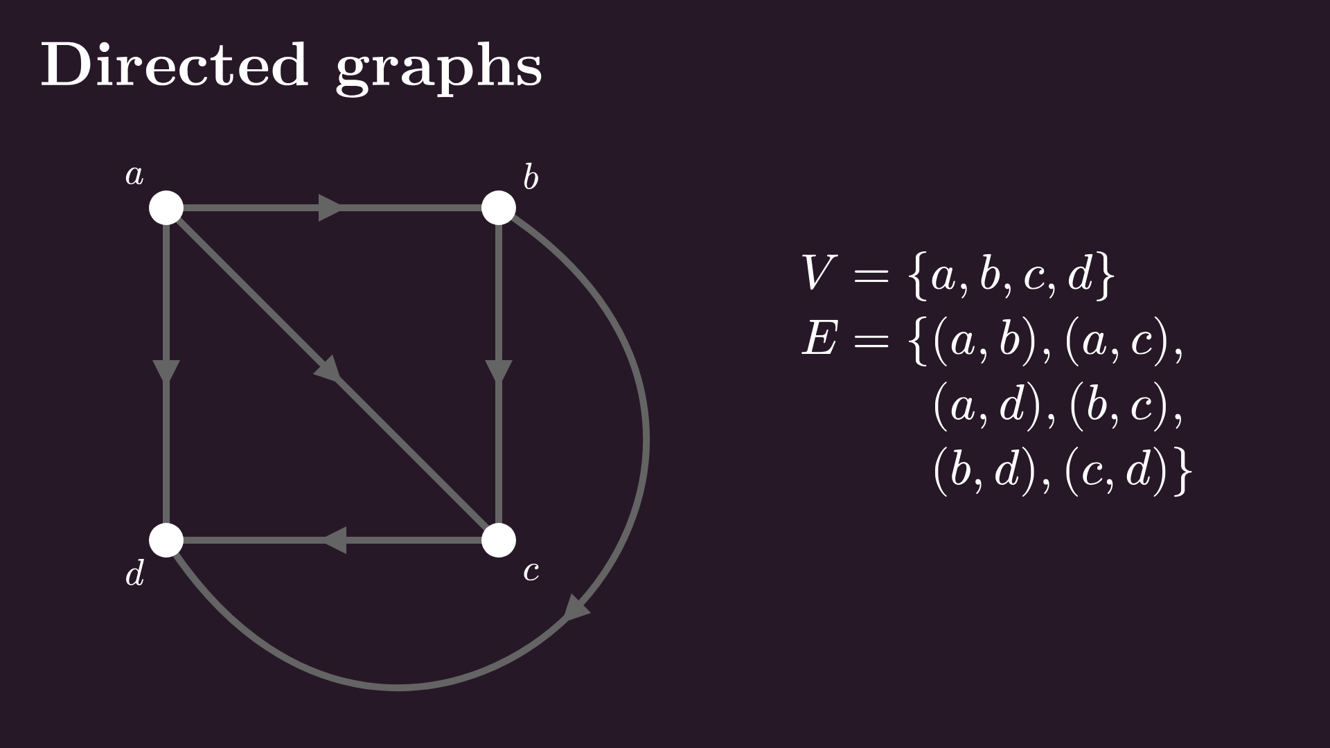
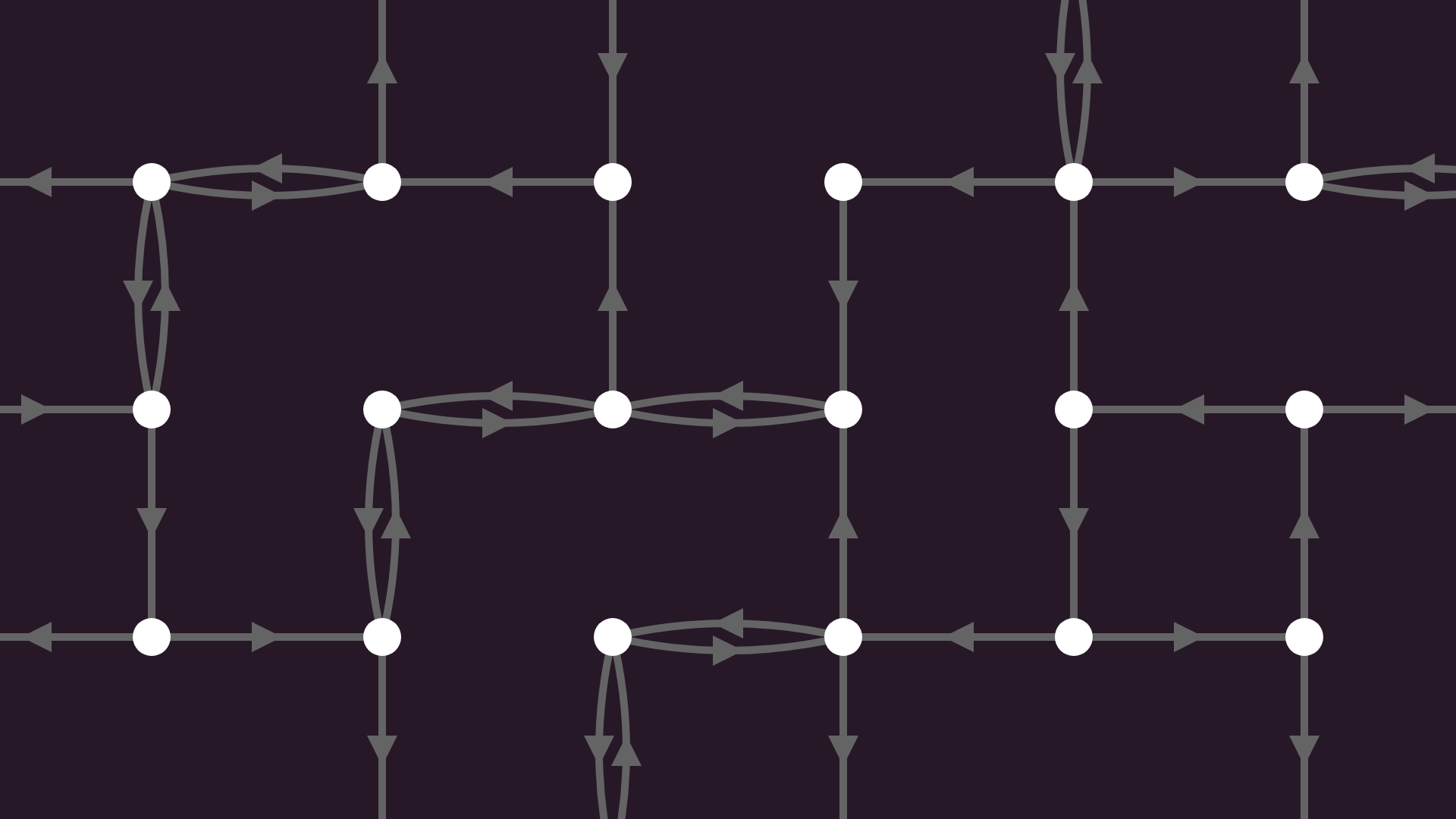
Directed graphs can be used to model all kinds of non-symmetric relations: the previously mentioned “a follows b” on social media, the “a links to b” on the internet, or the one-way connections between intersections in a city. In that case, nodes represent intersections, and directed edges represent one-way traffic lanes between them.
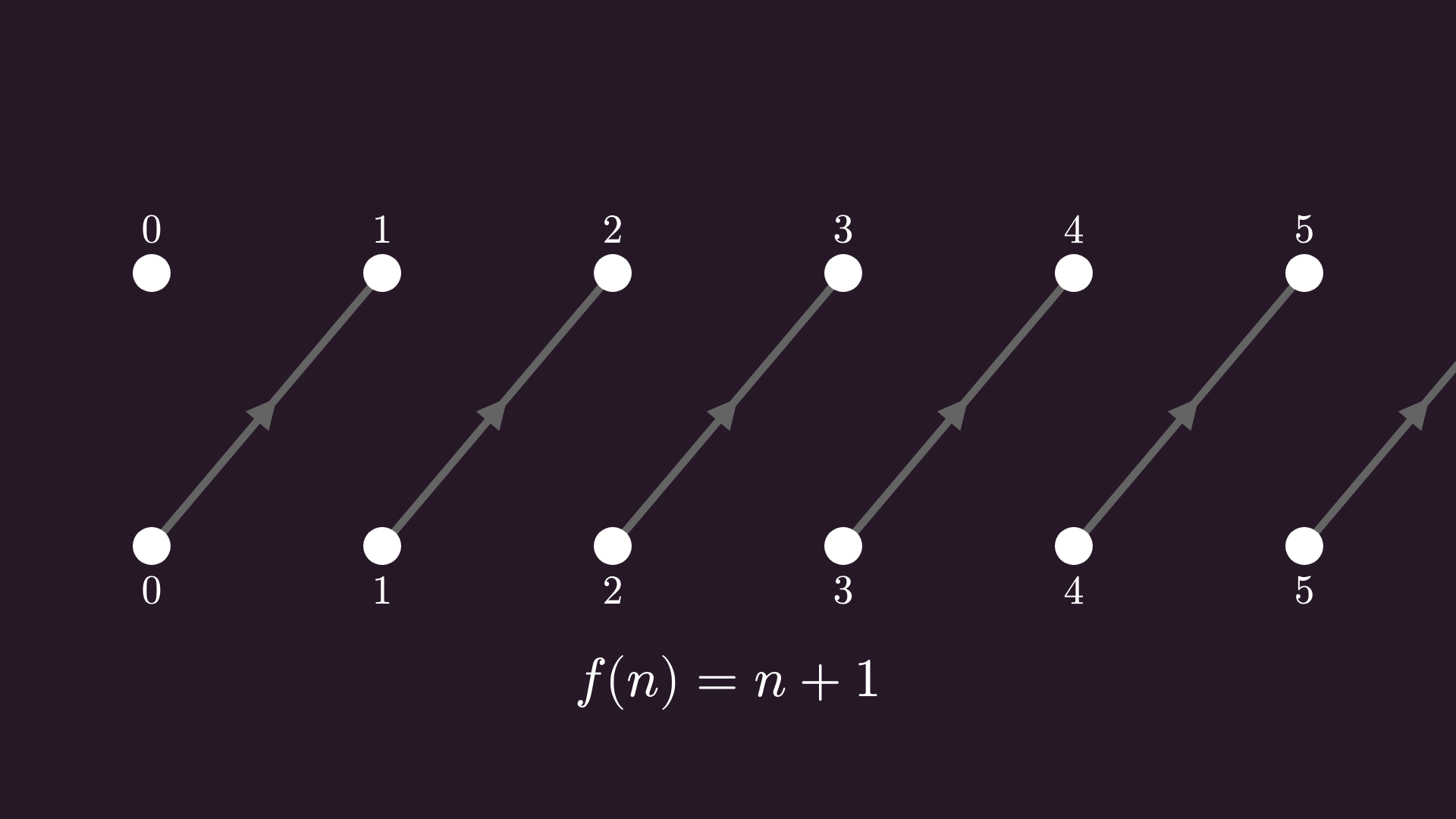
If you think about it, a function is a directed graph as well. Say, the function f(n) = n + 1 acting on the naturals can be thought of as an arrow from 0 to 1, an arrow from 1 to 2, and so on.
Speaking of functions: my favorite examples of graphs are computational graphs, that is, mathematical expressions in graph form. For instance, let’s take logistic regression, that is, the sigmoid function applied to ax + b.
A computer evaluates this expression in three steps, following the order of operations: first, a and x give ax by applying the multiplication operation; then, ax and b give ax + b via the addition operator; and finally, applying the sigmoid function to ax + b gives σ(ax + b).
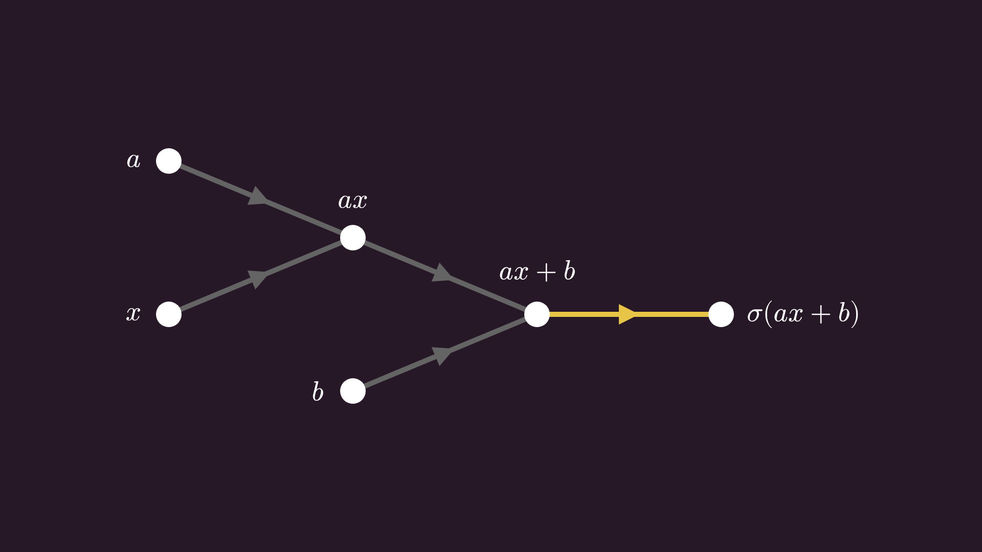
This is called a computational graph, representing variables as vertices and computational dependencies as edges. Neural networks, including the almighty large language models, are computational graphs, with potentially billions of nodes. However, to actually train a neural network, one needs the gradient of the computations, which is missing. If we store variables in nodes, it’s a natural idea to store gradients in the edges.
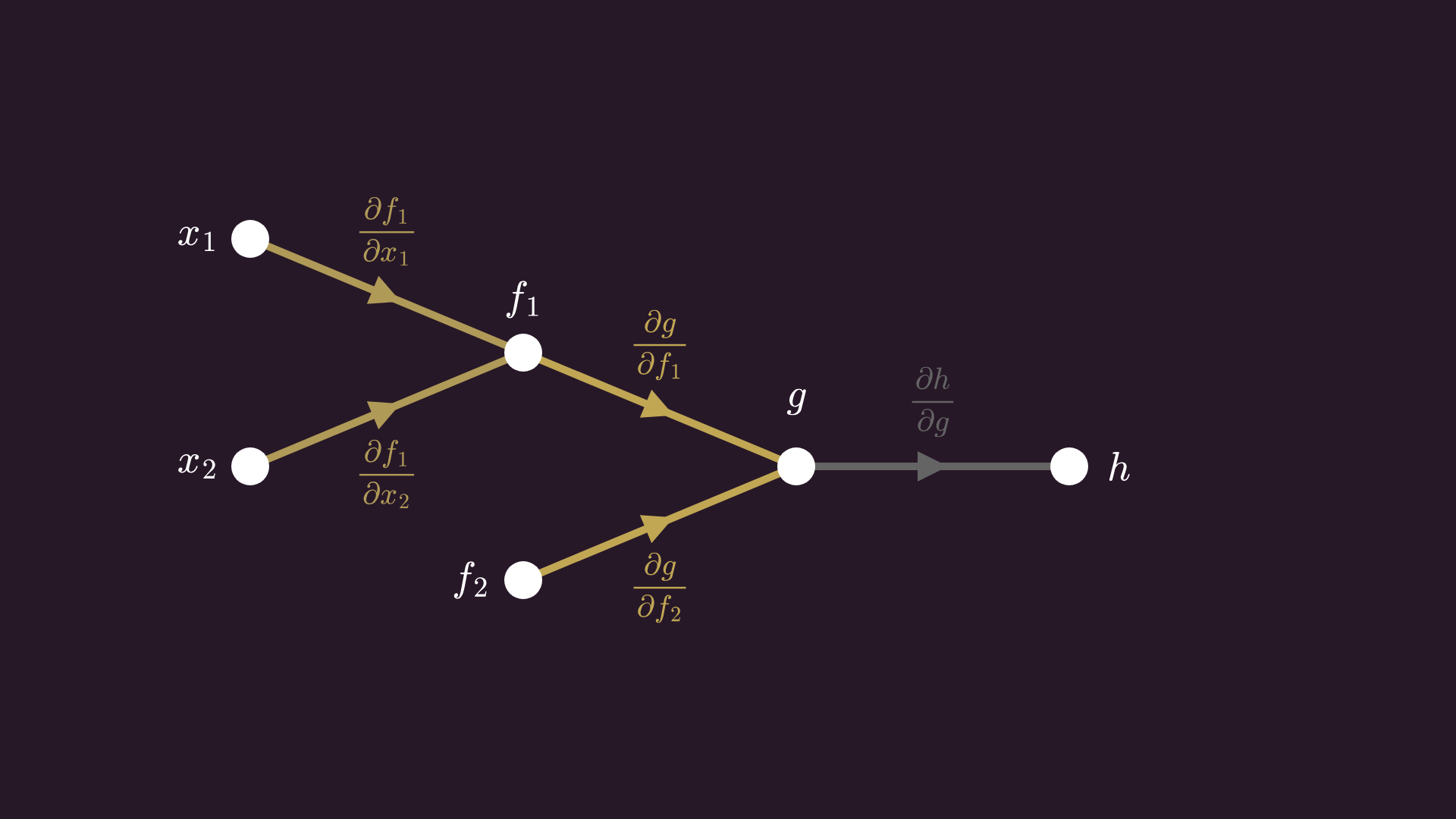
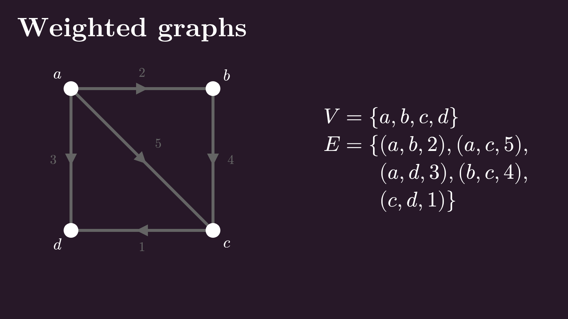
This gives us the motivation to introduce the concept of weighted graphs, allowing us to enhance the edges even further by giving them not only a direction but also a scalar value. Mathematically speaking, the weights are given by a function mapping the edges to scalars, but if you are closer to computer science, you might think of them as storing an extra value in the tuples representing the edges.
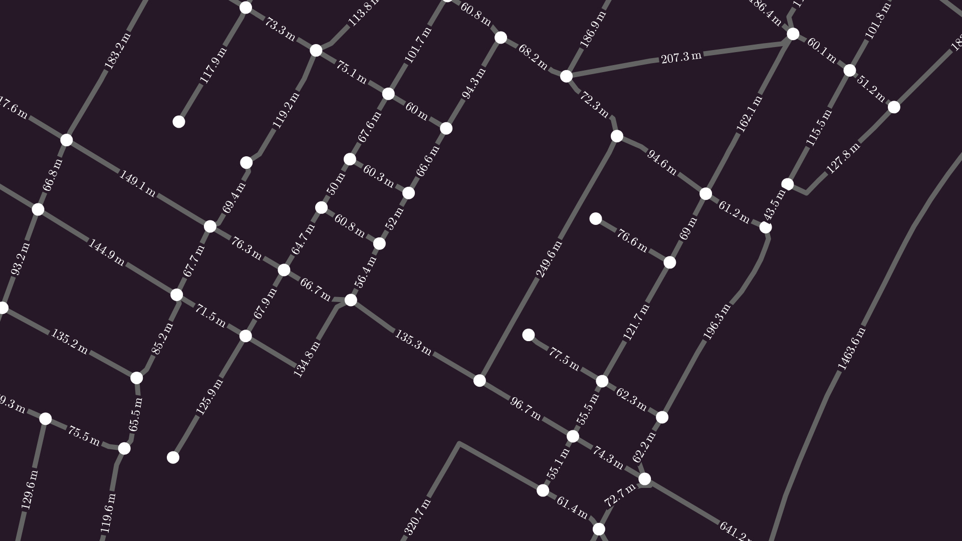
Weighted graphs are rich in applications besides computational graphs. For instance, recall the graph of my hometown we saw a while ago. It’s actually a weighted (but not directed) graph, storing the length of each street segment along the edges. When we compute shortest paths in this graph, we take the weights into account as well.
Another example. If you flip a coin to lose or win a dollar each time, you can track your profits on a simple plot, like what you are seeing right now.
We think about this as a function of (discrete) time, but in fact, we are simply randomly walking on a graph, taking a step in either direction with probability p = 0.5, with the probabilities serving as weights for our graph.
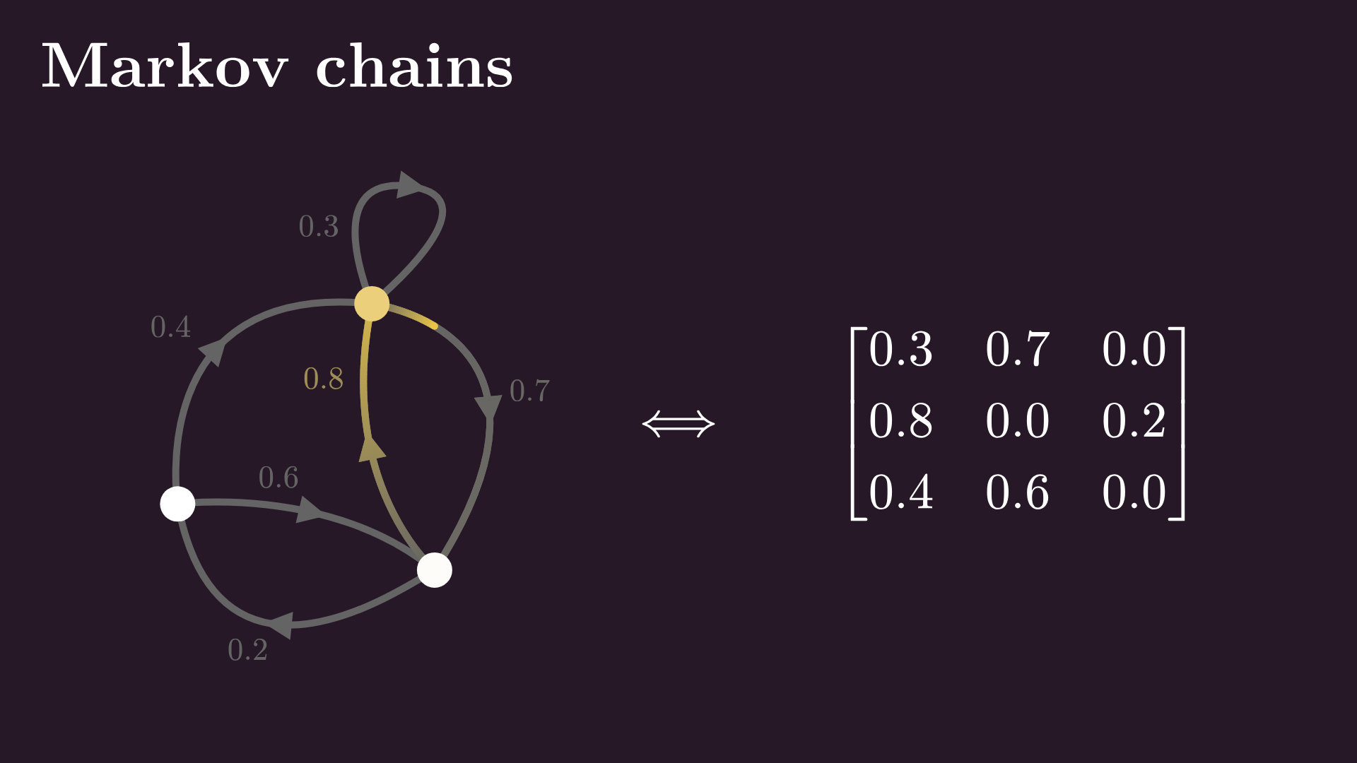
This idea of randomly walking around a directed graph is formalized by the concept of Markov chains. For instance, here’s a simple example with three nodes, called the transition graph of the Markov chain. At each node, we choose the next one according to the probability distribution determined by the outgoing weights.
By the way, this entire process is described via the so-called transition matrix. If we let go of probabilities and allow arbitrary weights, we obtain the adjacency matrix, providing a compact representation for directed and weighted graphs. I made a full video on this; check the link in the description. All in all, directed and weighted graphs are everywhere in mathematics, computer science, and science in general.
Graph measures
The last topic of our journey into graph theory ties perfectly into Markov chains. Let’s stop the random walk for a moment and ask the question: how much time does the process spend at each node in the long run? Let’s count it.
We’ll plot the proportion of time spent at each node on a histogram. By cranking up the speed, we can see the histograms settle, showing that the random walk spends most of its time at v₁, then at v₂, and only a small portion at v₃. This is called the equilibrium distribution of the graph, and surprise, surprise, this is exactly what Google’s famous PageRank algorithm computes on the graph of websites to measure the importance of each site.
This is just one example of a graph measure. I’ll talk about one more: centrality. For that, we’ll need a more complex example, so let’s revisit my hometown once more.
Let’s focus on this intersection inside suburbia. If we are travelling from A to B, how likely are we to cross this intersection below, marked with green?
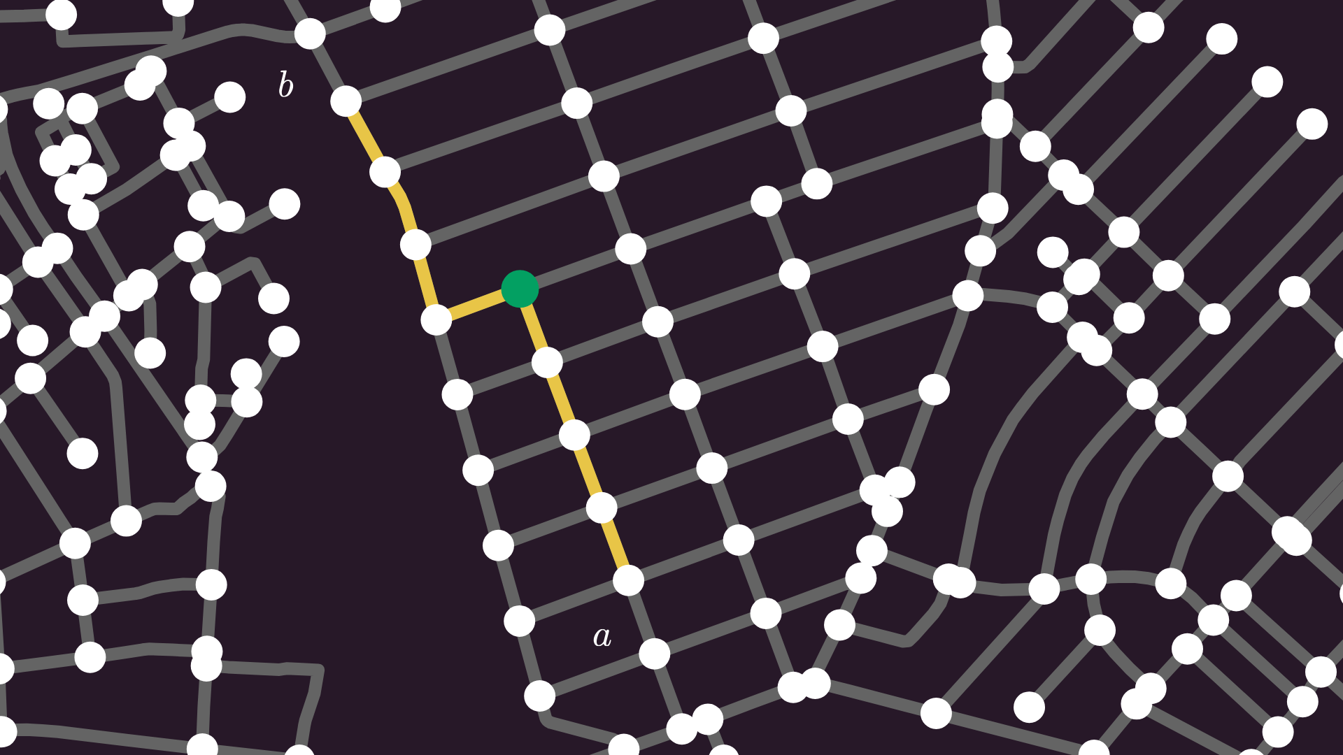
Let’s assume that we always select the shortest path. If we are moving inside the neighbourhood, then sure, the intersection in question might be on it, but otherwise, we are unlikely to cross it.
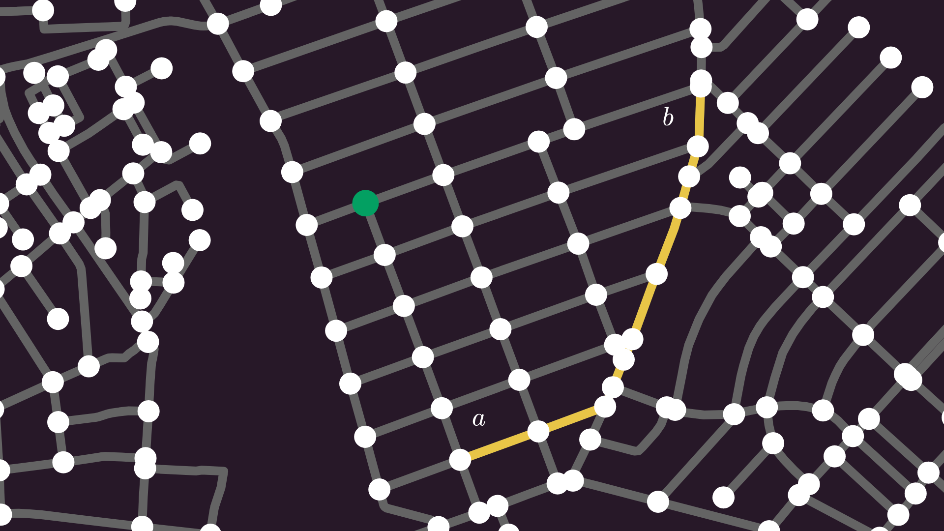
On the other hand, let’s check the intersection that leads to one of the two bridges. Many paths between the two halves of the city goes through this bridge, so compared to that obscure intersection in suburbia, you are unlikely to miss this one.
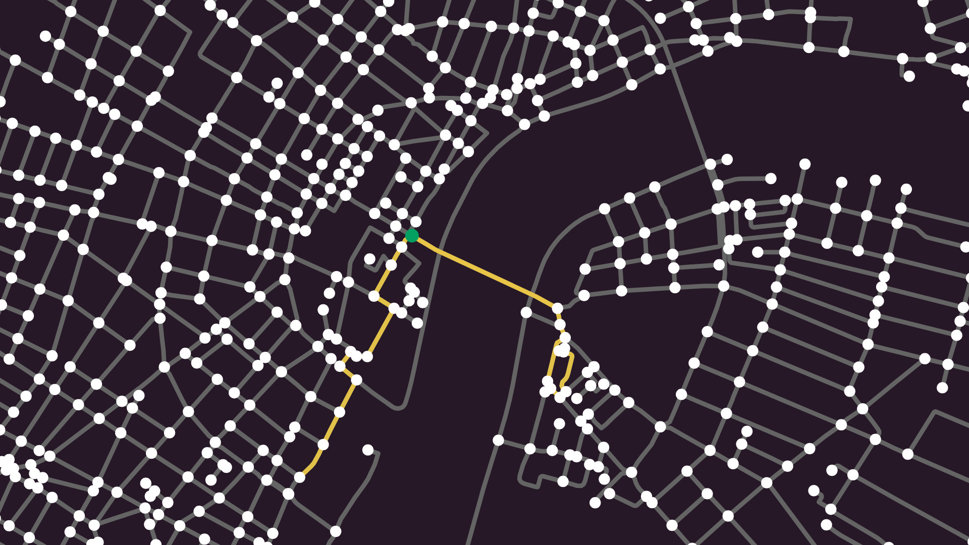
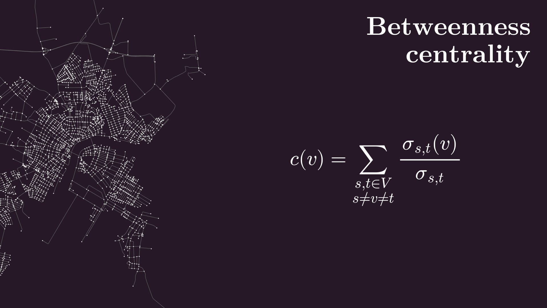
This idea is formalized by the concept of betweenness centrality, defined for any node v by this formula here: we count the shortest paths between s and t, take those that pass through v and compute their ratio, then sum for all s and t.
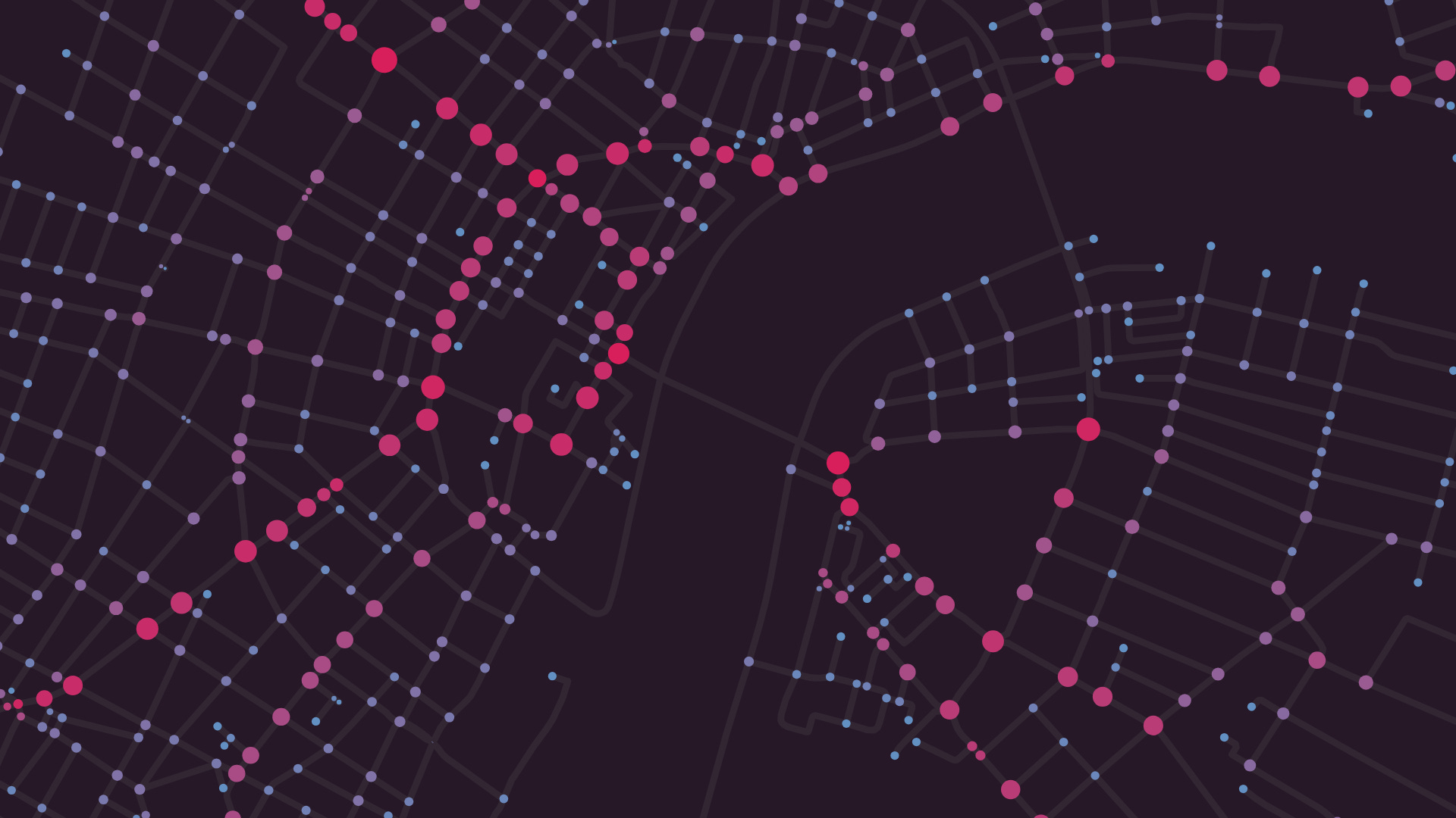
We can illustrate the centrality of each node by adjusting the vertex size and adding a blue-to-red colormap; blue is low centrality; red is high. The nodes around the bridges light up as expected.
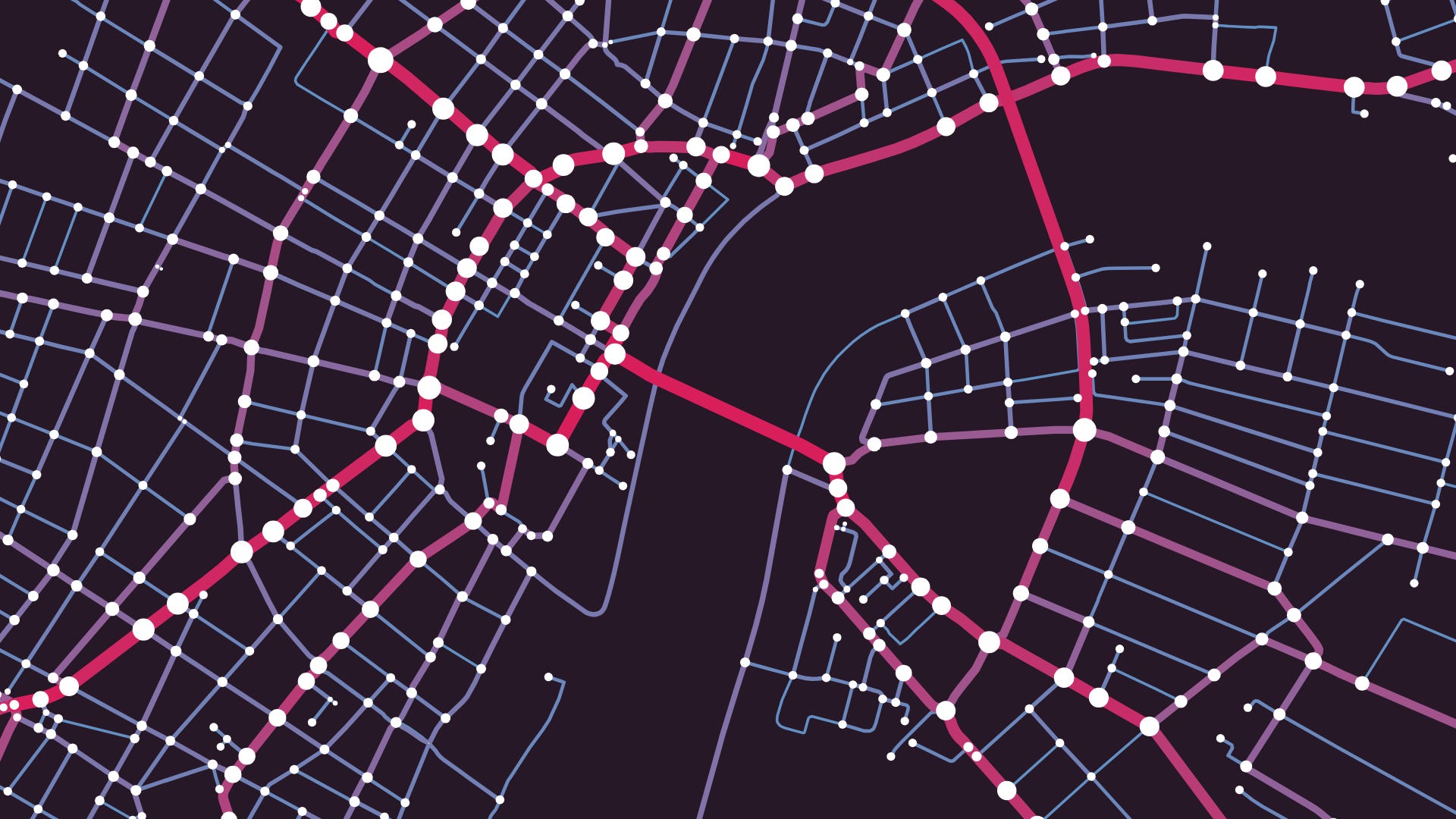
We can similarly define edge centrality, and overlaying that on top of our city graph completes the full picture. Without any traffic data, high-centrality nodes and edges help us identify potential bottlenecks. So now I have a theoretic justification to my avoidance of bridges.
Final thoughts
Graph theory is a rich subject, so we could continue our journey for a long time, but it’s time for us to wrap up. But before we leave, I would like to thank my channel members and Substack subscribers for your support. I’m an independent, audience-funded content creator, and your support makes videos such as this possible. Special thanks to the founding members of my Substack.
If you have enjoyed this post, like, subscribe, and consider supporting me via a paid membership! Thanks for reading, and see you soon!
Cheers,
Tivadar
Thanks for reading!
If you liked this post, please consider supporting me with a paid subscription. It’s $100 a year, or $10 a month, and in return you get well-researched machine learning/mathematics deep dives such as Machine Learning is Not Just Statistics, Matrices and Graphs, or Vectorization in Theory + Vectorization in Practice.
Your support makes it possible for me to write these high value, high signal posts.