Derivatives in One, Two, and a Billion Variables

A deep dive into differentiation

Quick note. There’s a -15% Black Friday deal for my Mathematics of Machine Learning book out there. Make sure to grab it!

---

Hi there!

Welcome to the next lesson of the Neural Networks from Scratch course, where we’ll build a fully functional tensor library (with automatic differentiation and all) in NumPy, while mastering the inner workings of neural networks in the process.

Check the previous lecture notes here:

1. Vectors and Matrices

2. Introduction to Computational Graphs

3. Computational Graphs in Python

In the last session, we finally dove deep into neural networks and implemented our first computational graphs from scratch.

Laying the groundwork for our custom neural-networks-from-scratch framework, we have implemented the Scalar class, representing computational graphs built by applying mathematical operations and functions. Something like this:

a = Scalar(1)
x = Scalar(2)
b = Scalar(3)

sigmoid(a * x + b) # <-- this is a computational graph

In essence, whenever we use a mathematical expression, say, to define a two-layer perceptron, we define a directed acyclic graph as well. This is called the forward pass, that is, the execution of our model.

To train the model, that is, find the weights that best fit our data, we have to perform parameter optimization with gradient descent. To perform gradient descent, we have to find the gradient. To find the gradient, we need to perform backpropagation, the premier algorithm for computing the derivatives of nodes in a computational graph.

Let’s start from scratch: what is the derivative?

The derivative

Mathematically speaking, computational graphs are functions, defined by expressions such as our recurring example of logistic regression, given by the function

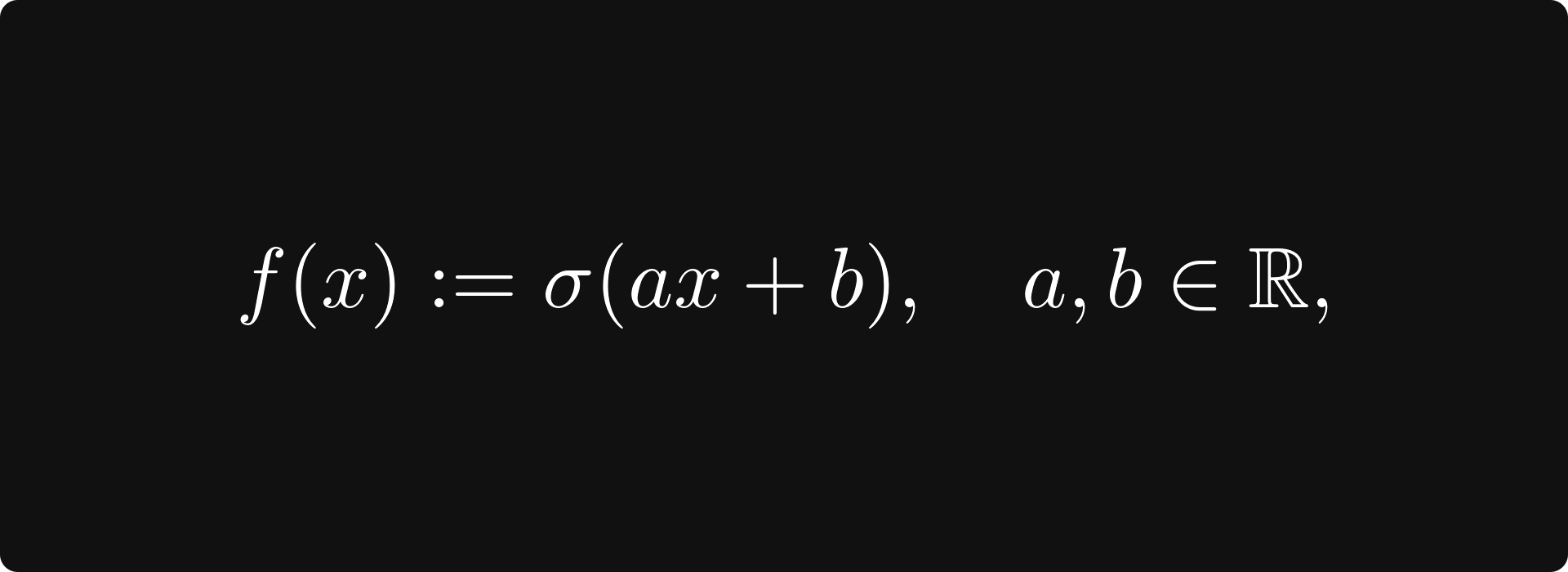
where x represents our measurements, and a, b represent the model parameters. This is where calculus comes into play.

To train a model, we combine it with a loss function — like the mean-squared error — and minimize the loss: if x₁, x₂, …, xₙ are our training data samples with labels y₁, y₂, …, yₙ, then the mean-squared error is given by the bivariate function

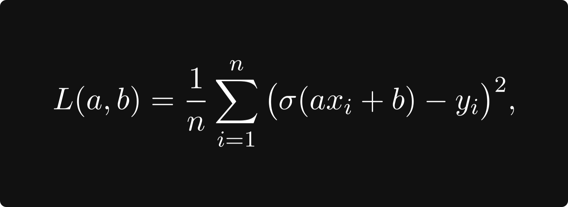
which is a function of the model parameters a and b.

How do we minimize the loss, that is, find the minimum of L(a, b)?

One idea is to measure the rate of change of L with respect to the variables a and b, then take a small step in the direction that decreases the loss. This is called gradient descent.

That’s good to know! But how do we measure the rate of change?

With the derivative. I’ll explain.