The Derivatives of Computational Graphs
Part 1. Forward-mode differentiation and its shortcomings
The single most undervalued fact of mathematics: matrices mathematical expressions are graphs, and graphs are matrices.
Yes, I know. You already heard this from me, but hear me out. Viewing neural networks — that is, complex mathematical expressions — as graphs is the idea that led to their success.
Computationally speaking, decomposing models into graphs is the idea that fuels backpropagation, the number one algorithm used to calculate the function's gradient. In turn, this gradient is used to optimize the model weights, a process otherwise known as training.
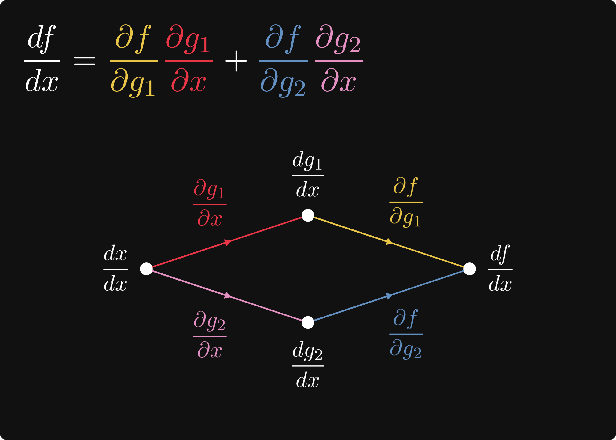
Take a look at this illustration below: this is the omnipotent chain rule in computational graph form.
This post is dedicated to explaining exactly what's going on in this picture.
So, you want to compute the derivatives of computational graphs. To make things concrete, we'll use a familiar example, the logistic regression.
In mathematical terms, logistic regression is defined by the function
where x is the input, and a, b are the model parameters. Our ultimate goal is to compute the rate of change of f with respect to the parameters a and b; that is, the derivatives ∂f/∂a and ∂f/∂b.
How to do that? Experienced calculus users immediately reply
but how was that obtained? By the chain rule, one of the most important results in mathematics. However, to fully understand what the chain rule is, we have to dive deep into the wonderful (and mildly convoluted) world of derivatives.
This post is the fourth part of my Neural Networks from Scratch series. Although I aim for every post to be self-contained, check out the previous episodes to get you up to speed.
Episode 1: Introduction to Computational Graphs
Episode 2: Computational Graphs as Neural Networks
Episode 3: Computational Graphs and the Forward Pass
Derivatives and partial derivatives
At some point in your life, you have probably encountered the concept of differentiation and derivatives. We don't have all the time in the world here, but let's recap; it's best if we tackle the tough topic of backpropagation fully prepared.
In pure English, derivatives describe the rate of change. Let's see the formal definition.
Definition. (The derivative.) Let f: ℝ → ℝ be a function of one variable. We say that f is differentiable at x₀ if the limit
exists. If so, df/dx(x₀) is called the derivative of f at x₀. If f is differentiable everywhere, then it is said to be differentiable.
Two remarks about the notation. First, when it's clear, the argument is omitted from the so-called Leibniz notation df/dx = df/dx(x₀).
Second, for univariate functions, the derivate is also denoted by f′(x₀); we'll use this quite frequently.
Geometrically speaking, the f′(x₀) describes the slope of the tangent line drawn at the graph of f at the point (x₀, f(x₀)).
It's the best to visualize this, so we'll take a look at the function f(x) = x², whose derivative is f′(x) = 2x.
However, in multiple variables, the definition breaks down. For instance, consider
f(x, y) = x² + y², the two-variable version of the previous function. There, instead of a tangent line, we have a tangent plane.
In this case, we can fix all but one variable, and take the derivative of the thus obtained single-variable function. This is called the partial derivative. Here's the formal definition.
Definition. (The partial derivative.) Let f: ℝⁿ → ℝ be a function of n variables. We say that f is partially differentiable at 𝐱₀ in the i-th variable if the limit
exists, where 𝐞ᵢ is the vector whose i-th coordinate is one, and the rest is zero. If so,
∂f/∂xᵢ(𝐱₀) is called the i-th partial derivative of f at 𝐱₀.
Again, when it's clear, we often write ∂f/∂xᵢ instead of ∂f/∂xᵢ(𝐱₀).
Let's look at an example! In the case of f(x, y) = x² + y³, the partial derivatives are
I want to make a remark here. When vigorously composing functions and variables (as we do in machine learning), a clear distinction must be made between regular and partial derivatives. For example, consider the functions f(x, y) = x + y² and g(x, y) = sin(x) cos(y). If x and y represent a particular feature like height, cost, etc., and g(x, y) is an engineered feature, we end up with expressions like
In this context, df/dy and ∂f/∂y mean two different things:
while ∂f/∂y is the partial derivative of f with respect to y,
the expression df/dy refers to the univariate function defined by y → f(g(x, y), y), or in other words, df/dy = ∂h/∂y.
Keep this in mind, as we won't always explicitly name composite expressions such as f(g(x, y), y).
Speaking of composed functions: it's time to dive into the chain rule, our main tool for differentiating computational graphs.
The chain rule
Let's state the chain rule right away. Single variable first, multiple variables second.
Theorem. (Chain rule, single variable.) Let f, g: ℝ→ℝ be two differentiable functions, and let h(x) = f(g(x)). Then
or in other words,
In English, this means that the derivative of the composite function equals the product of the components' derivatives, evaluated at the appropriate locations.
If you are an attentive reader, perhaps you've noticed that there's a discrepancy between the notations f′(g(x)), df/dx, df/dg, and so on.
For instance, df/dx and df/dg doesn't make sense, as the function f is univariate, defined in terms of an arbitrary variable x. So, what's df/dg? Let's clear this up once and for all.
According to the chain rule, the derivative of the composed function f(g(x)) is
in other words, the derivative function f′ is evaluated at g(x). To avoid writing monstrosities like df/dx(g(x)), we rather think of f as defined in terms of the variable g = g(x), and simply write df/dg, which is shorthand for
For multiple variables, the chain rule goes like the following.
Theorem. (Chain rule, multiple variables.) Let
f: ℝᵐ → ℝ be a function of m variables,
g₁, ..., gₘ: ℝⁿ → ℝ be functions of n variables,
and define h: ℝⁿ → ℝ by
Then
How does this apply to the logistic regression? As we've seen that before, f(a, b, x) = σ(a x + b) is a composite function, built from the blocks
that yield
Thus,
as we've seen it earlier.
Because of the layered structure of neural networks, the chain rule will be our bread and butter in calculating the derivatives. Now that we understand how it works, let's see what the chain rule means in the context of computational graphs!
Tired of dense textbooks and confusing jargon?
The Palindrome breaks down advanced math and machine learning concepts with visuals that make everything click.
Join the premium tier to get instant access to guided tracks on graph theory, foundations of mathematics, and neural networks from scratch.
The chain rule and computational graphs
Let's go back to square one and consider the composite function f(g(x)). In computational graph terms, we prefer to work with variables, not functions. That is, instead of f(g(x)), we have the variables x, g, f, the elements of our computations.
Here's how this simple graph looks.
Note that in the above computational graph, g
is not the mathematical function g, nor does f
mean f. The variables are the results of the computations defined by the functions. Mathematically speaking, we have
the input x,
the variable
g
= g(x),and the variable
f
= f(g).
In principle, we are not allowed to designate the same symbol to different variables, but adding another set of symbols would be cumbersome. Thus, we take a hit in precision to gain a bit of simplicity.
Accordingly,
df/dx is the derivative of f(g(x)) with respect to x,
while df/dg is the derivative of f with respect to its only variable g.
Keep this in mind when translating expressions to computational graphs.
In the language of computational graphs, the chain rule expresses the derivative of the terminal node f
with respect to the initial node x
. Essentially, we compute the following graph.
This is quite overloaded with information, so let me explain. In the derivative graph,
a node corresponds to the derivative of the original node with respect to the initial node
x
,and an edge corresponds to the derivative of its end node with respect to its start node.
Using the chain rule, we obtain the values in the nodes by multiplying together all the edges leading up to it:
Because we progress from the initial node x
to the terminal node f
, this is called forward-mode differentiation. Accordingly, the
derivatives represented by the nodes are called the forward derivatives,
and the derivatives on the edge are called local derivatives.
Let's see an example to solidify your understanding: consider the expression (3x)². In this setting, g(x) = 3x and f(g) = g². Thus, we have
For, say, x = 4, we can immediately compute the forward pass and the local derivatives:
Thus, in the first step, we populate the edges and the first node of the derivative graph.
The second node is computed by taking the product of the first node and the first edge. (As the first node's value is 1, this'll match the edge.)
In the last step, we compute df/dx by taking the product of df/dg = 24 and dg/dx = 3.
To get a firm grasp on how forward-mode differentiation works, let's put one more node and consider the graph given by h(f(g(x))).
To check your understanding, try to carry through the previous process by
sketching the derivative graph,
and computing the derivatives of the nodes with respect to the initial node
x
.
Welcome back! This is what you should have got:
To confirm, the iterated application of the chain rule gives
Now you understand why the chain rule is called the chain rule! The next step is see what happens in a multivariable context.
The multivariable case
Let's turn the difficulty dial up a notch and consider the expression
which is composed of
a bivariate function f: ℝ² → ℝ,
and two univariate functions g₁, g₂: ℝ → ℝ.
Sketching up its graph, we obtain the following.
Again, our goal is to calculate df/dx. To do that, we employ the (multivariate) chain rule
or in computational graph terms:
(Note that here,
holds.) In this case, the derivative df/dx is obtained via forward-mode differentiation; that is,
1. computing the local derivatives on the edges,
2. taking a path from the initial node x
to the terminal node f
,
3. multiplying together all intermediate derivatives along the edges,
4. and summing the products for all paths.
Take a look at the expression
where the first term (∂f/∂g₁) ⋅ (∂g₁/∂x) corresponds to the left path, while (∂f/∂g₂) ⋅ (∂g₂/∂x) corresponds to the right one.
From top to bottom, we compute
dx/dx,
dg₁/dx and dg₂/dx,
and finally df/dx,
in this exact order.
Like before, we'll walk through a concrete example: sin(x) cos(x). This expression is a composition of two univariate functions g₁(x) = sin(x), and g₂(x) = cos(x), and a bivariate function f(g₁, g₂) = g₁ ⋅ g₂. Regarding its derivatives, we have
and
So, what would calculating the derivative look like for, say, x = 2? Let's begin populating the derivative graph with the edges and the first node.
With this, we can move one step further and compute the derivatives of the first-level nodes.
The final step. According to the chain rule, the derivative is the sum of the values of all the incoming edges times their parents' derivative for each node. In simpler terms,
which is the following in graph form:
If you want to practice, feel free to carry out the previous process on the expression cos(x²) sin(x²).
One more example to emphasize the difference between local derivatives ∂/∂x and global derivatives d/dx. Let's put one more layer into the above graph and consider the expression
yielding the following (derivative) graph.
Here, the chain rule says that
Note that the terms (∂f/∂gᵢ) ⋅ (∂gᵢ/∂hᵢ) ⋅ (∂hᵢ/∂x) correspond to paths from x
to f
, while (∂f/∂gᵢ) ⋅ (dgᵢ/dx) correspond to all incoming edges and parents of f
.
Now, it's time to put a twist on everything that we've learned so far regarding the chain rule!
The problems with forward-mode differentiation
Let's increase the complexity once more and consider the computational graph defined by the expression
which looks like the following.
As there are two initial nodes x₁ and x₂, we would like to compute both df/dx₁ and df/dx₂. This presents us with a problem, as now we have to compute two graphs:
(I have omitted the edge labels for clarity.)
Now, our computational cost has increased twofold. For n input variables (or features), the increase is n-fold. In practice, the number of input variables is in the millions. (Depending on which year you read this, it might even be in the billions.) This is a significant issue if we were to calculate the derivatives this way.
That's only the tip of the iceberg. Next, consider an analogous computational graph coming from the expression
This time, there are three input nodes (x₁
, x₂
, x₃
) and three middle nodes (g₁
, g₂
, g₃
).
The number of paths from initial to terminal nodes increases dramatically with adding new nodes. Compared to f(g₁(x₁, x₂), g₂(x₁, x₂)) , where we had only 2 ⋅ 2 = 4 paths, this time, we have 3 ⋅ 3 = 9.
This gets exponentially worse if we add another layer. Consider the following computational graph. (I don't even want to show you the expression it came from, let alone type it.)
The number of paths to sum over has gone from 3² to 3³ = 27. This is the dreaded exponential increase.
What can we do? Enter the backward-mode differentiation, which we’ll dissect in the next post.
See you there!
When you’re ready, here’s how I can help further:
Upgrade to the paid tier to access the learning tracks on graph theory, foundations of mathematics, and neural networks from scratch.
The Mathematics of Machine Learning book is out now! Grab a copy here and master linear algebra, calculus, and probability theory for ML. Bridge the gap between theory and real-world applications, and learn Python implementations of core mathematical concepts.