Why does gradient descent work?
Rolling downhill with dynamical systems
Young man, in mathematics you don’t understand things.
You just get used to them. — John von Neumann
In machine learning, we use gradient descent so much that we get used to it. We hardly ever question why it works.
What's usually told is the mountain-climbing analogue: to find the peak (or the bottom) of a bumpy terrain, one has to look at the direction of the steepest ascent (or descent) and take a step towards there. This direction is described by the gradient, and the iterative process of finding local extrema by following the gradient is called gradient ascent/descent. (Ascent for finding peaks, descent for finding valleys.)
However, this is not a mathematically precise explanation. Several questions are left unanswered, and based on our mountain-climbing intuition, it's not even clear if the algorithm works.
Without a precise understanding of gradient descent, we are practically flying blind. In this post, our goal is to develop a proper mathematical framework that will help you understand what's going on behind the scenes. This will allow you to effectively reason about gradient descent, and possibly improve its performance in your projects. Our journey is leading us through
differentiation, as the rate of change,
the principles of optimization with first and second derivatives,
the basics of differential equations,
and how gradient descent is equivalent to physical systems flowing towards their equilibrium state.
Buckle up! Deep dive into the beautiful world of dynamical systems incoming.
Derivatives and their meaning
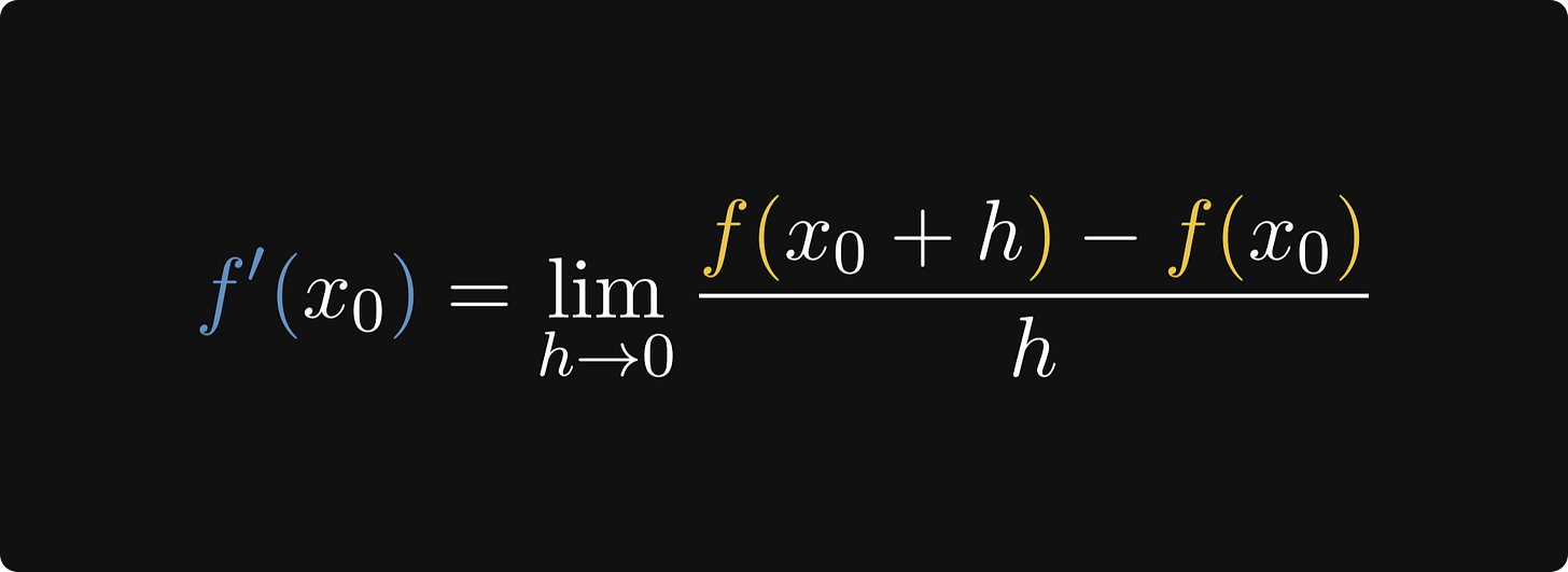
If you are comfortable with the gradient descent algorithm, we can start to peek behind the curtain. Let's talk about derivatives first! By definition, we say that a function f is differentiable at x₀ if the limit
exists. f ′(x₀) is called the derivative. Although this definition seems random, there is a deep meaning behind it: the derivative can be thought of as the rate of change.
Derivative as speed
Let's jump back in time a few hundred years! At its inception, derivatives were created to describe the speed of moving objects. Suppose that the position of our object at time t is given by the function x(t), and for simplicity, assume that it is moving along a straight line—something like this below.
Our goal is to calculate the object's speed at a given time. In high school, we learned that
To put this into a quantitative form, if t₀ < t₁ are two arbitrary points in time, then
Expressions like x(t₁) - x(t₀) are called differential quotients. Note that if the object moves backwards, the average speed is negative.
The average speed has a simple geometric interpretation. If you replace the object's motion with a constant velocity motion moving at the average speed, you'll end up at the same place. In graphical terms, this is equivalent of connecting (t₀, x(t₀)) and (t₁, x(₁)) with a single line. The average speed is just the slope of this line.
Given this, we can calculate the exact speed at a single time point t₀. The idea is simple: the average speed in the small time-interval between t₀ and t₀ + Δt should get closer and closer to the exact speed at t₀ if Δt is small enough. (Δt can be negative as well.)
Thus,
Geometrically, you can visualize the derivative as the tangent line at t₀, and the differential quotients as slopes of the lines connecting the function's graph between t₀ and t₀ + Δt.
Local extrema and the derivative
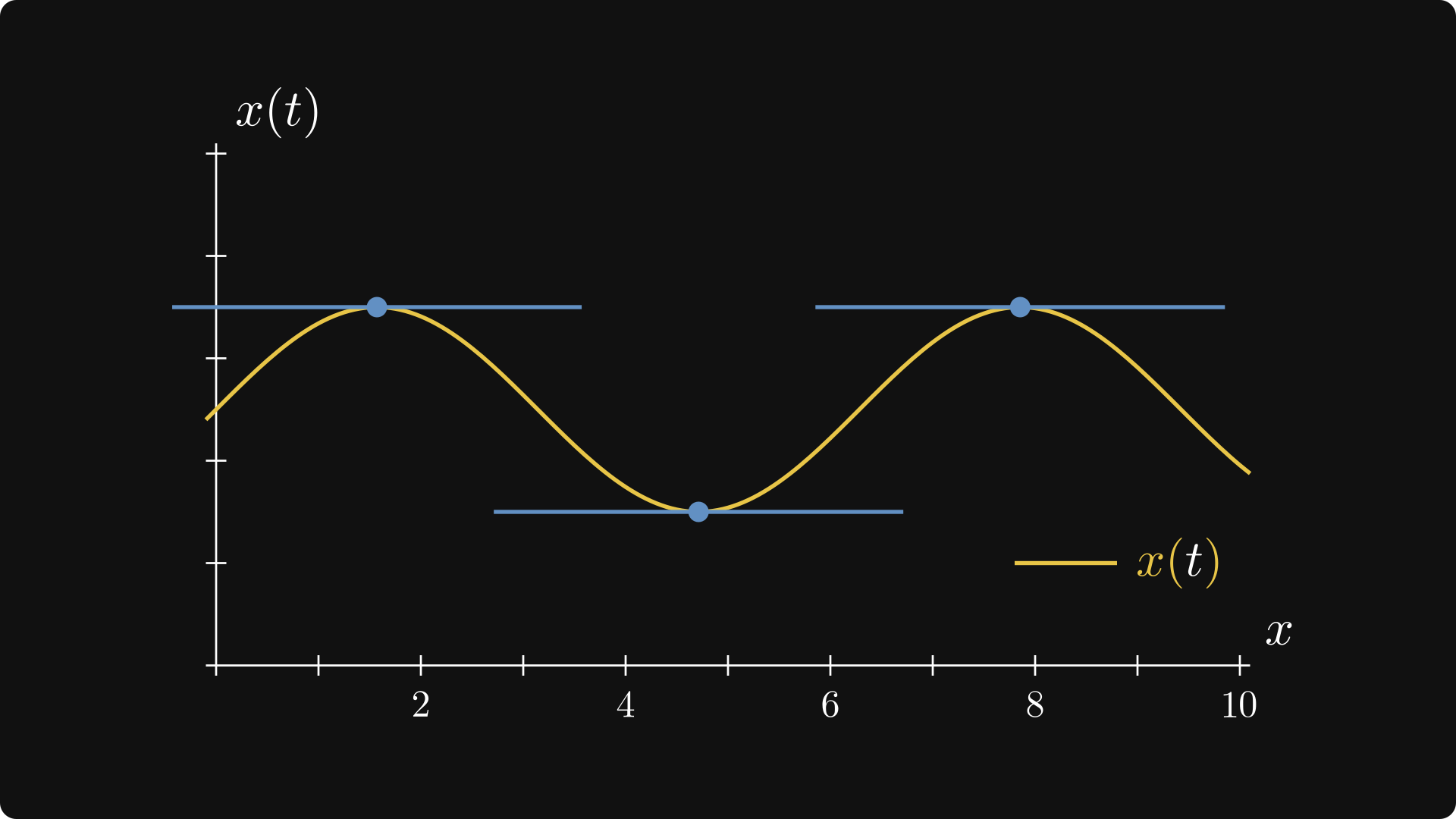
Derivatives can tell us a lot more than speed. We've just seen that the derivative equals the slope of the tangent line. With this in mind, take a look at the figure below!
Notice that the tangent is perfectly horizontal at the local minima and maxima. In mathematical terms, this is equivalent to x′(t) = 0. Can we use this property to find minima and maxima?
Yes, but it's not that simple. Take a look at x(t)=t³. Its derivative is zero at 0, but that is not a local minimum nor a local maximum. Without going into the fine details, the best we can do is to compute the second derivative and hope that it'll give some clarity. To be precise, the following theorem holds.
Why is this important to us? Well, because machine learning is (mostly) just a colossal optimization problem. Construct a parametric model, and find a set of parameters that maximize its performance. As you know, this is done via the famous gradient descent algorithm, which seemingly has nothing to do with our simple result regarding the second derivatives. However, quite the opposite is true: deep down at its core, this stems from the relation of local extrema and the first two derivatives.
In the following, we are going to learn why.
Differential equations 101
What is a differential equation?
Equations play an essential role in mathematics. This is common wisdom, but there is a profound truth behind it. Quite often, equations arise from modeling systems such as interactions in a biochemical network, economic processes, and thousands more. For instance, modeling the metabolic processes in organisms yields linear equations of the form
where the vectors x and b represent the concentration of molecules (where x is the unknown), and the matrix A represents the interactions between them. Linear equations are easy to solve, and we understand quite a lot about them.
For instance, the trajectory of a swinging pendulum can be described by the equation
where
x(t) describes the angle of the pendulum from the vertical,
L is the length of the (massless) rod that our object of mass m hangs on,
and g is the gravitational acceleration constant ≈ 9.7m/s².
According to the original interpretation of differentiation, if x(t) describes the movement of the pendulum at time t, then x′(t) and x′′(t) describe the velocity and the acceleration of it, where the differentiation is taken with respect to the time t.
(In fact, the differential equation of the swinging pendulum is a direct consequence of Newton's second law of motion.)
Equations involving functions and their derivatives, such as the equation of the swinging pendulum above, are called ordinary differential equations, or ODEs in short. Without any overexaggeration, their study has been the primary motivating force of mathematics since the 17th century. Trust me when I say this, differential equations are one of the most beautiful objects in mathematics. As we are about to see, the gradient descent algorithm is, in fact, an approximate solution of differential equations.
The first part of this post will serve as a quickstart to differential equations. I will mostly follow the fantastic Nonlinear Dynamics and Chaos book by Steven Strogatz. If you ever desire to dig deep into dynamical systems, I wholeheartedly recommend this book to you. (This is one of my favorite math books ever. It reads like a novel. The quality and clarity of its exposition serve as a continuous inspiration for my writing.)
The (slightly more) general form of ODEs
Let's dive straight into the deep waters and start with an example to get a grip on differential equations. Quite possibly, the simplest example is the equation
where the differentiation is taken with respect to the time variable t. If, for example, x(t) is the size of a bacterial colony, the equation x′(t) = x(t) describes its population dynamics if the growth is unlimited. Think about x′(t) as the rate at which the population grows: if there are no limitations in space and nutrients, every bacterial cell can freely replicate whenever possible. Thus, since every cell can freely divide, the speed of growth matches the colony's size.
In plain English, the solutions of the equation x′(t) = x(t) are functions whose derivatives are themselves. After a bit of thinking, we can come up with a family of solutions:
(Recall that the exponential is an elementary function, and its derivative is itself.)
Some of the solutions are plotted below.
There are two key takeaways here: differential equations describe dynamical processes that change in time, and they can have multiple solutions. Each solution is determined by two factors: the equation itself, and an initial condition x(0) = x*. If we specify x(0) = x*, then the value of c is given by
Thus, ODEs have a bundle of solutions, each one determined by the initial condition. So, it's time to discuss differential equations in more general terms! Here is the precise definition.
When it is clear, the dependence on t is often omitted, so we only write x′ = f(x).
The term "first-order homogeneous ordinary differential equation" doesn't exactly roll off the tongue, and it is overloaded with heavy terminology. So, let's unpack what is going on here.
The differential equation part is clear: it is a functional equation that involves derivatives. Since the time t is the only variable, the differential equation is ordinary. (As opposed to differential equations involving multivariable functions and partial derivatives, but more on those later.) As only the first derivative is present, the equation becomes first-order. Second-order would involve second derivatives, and so on. Finally, since the right-hand side f(x) doesn't explicitly depend on the time variable t, the equation is homogeneous in time. Homogeneity means that the rules governing our dynamical system don't change over time.
Don't let the f(x(t)) part scare you! For instance, in our example x′(t) = x(t), the role of f is cast to the identity function f(x) = x. In general, f(x) establishes a relation between the quantity x(t) (which can be position, density, etc.) and its derivative, that is, its rate of change.
As we have seen, we think in terms of differential equations and initial conditions that pinpoint solutions among a bundle of functions. Let's put this into a proper mathematical definition!
Most often, we select t₀ to be 0. After all, we have the freedom to select the origin of the time as we want.
Unfortunately, things are not as simple as they seem. In general, differential equations and initial value problems are tough to solve. Except for a few simple ones, we cannot find exact solutions. (And when I say we, I include every person on the planet.) In these cases, there are two things that we can do: either we construct approximate solutions via numerical methods or turn to qualitative methods that study the behavior of the solutions without actually finding them.
We'll talk about both, but let's turn to the qualitative methods first. As we'll see, looking from a geometric perspective gives us a deep insight into how differential equations work.
A geometric interpretation of differential equations
When finding analytic solutions is not feasible, we look for a qualitative understanding of the solutions, focusing on the local and long-term behavior instead of formulas.
Imagine that given a differential equation x′(t) = f(x(t)), you are interested in a particular solution that assumes the value x* at time t₀. For instance, you could be studying the dynamics of a bacterial colony and want to provide a predictive model to fit your latest measurement x(t₀) = x*. In the short term, where will your solutions go?
We can immediately notice that if x(t₀) = x* and f(x*) = 0, then the constant function
x(t) = x* is a solution! These are called equilibrium solutions, and they are extremely important. So, let's make a formal definition!
Think about our recurring example, the simplest ODE x′(t) = x(t). As mentioned, we can interpret this equation as a model of unrestricted population growth under ideal conditions. In that case, f(x) = x, and this is zero only for x = 0. Therefore, the constant x(t) = 0 function is a solution. This makes perfect sense: if a population has zero individuals, no change is going to happen in its size. In other words, the system is in equilibrium.
Like a pendulum that stopped moving and reached its resting point at the bottom. However, pendulums have two equilibria: one at the top and one at the bottom. (Let's suppose that the mass is held by a massless rod. Otherwise, it would collapse) At the bottom, you can push the hanging mass all you want, it'll return to rest. However, at the top, any small push would disrupt the equilibrium state, to which it would never return.
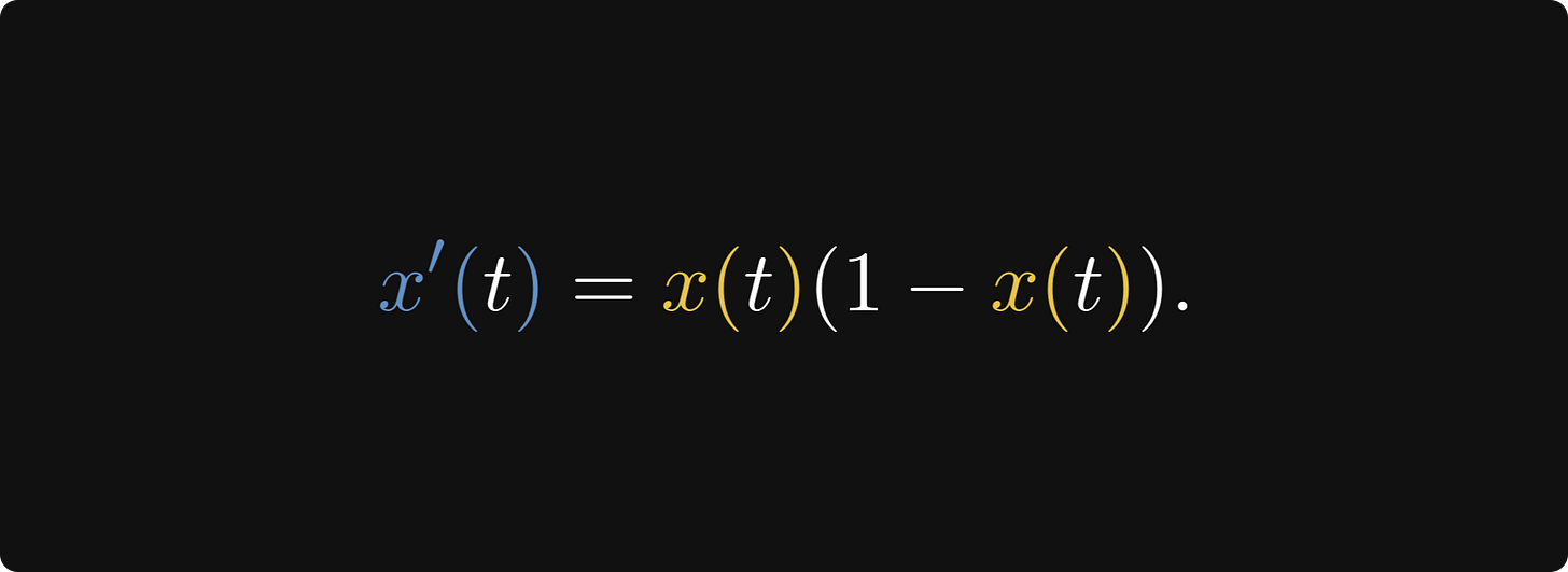
To shed light on this phenomenon, let's look at another example: the famous logistic equation
From a population dynamics perspective, if our favorite equation x′(t) = x(t) describes the unrestricted growth of a bacterial colony, the logistic equation models the population growth under a resource constraint. If we assume that 1 is the total capacity of our population, the growth becomes more difficult as the size approaches this limit. Thus, the population's rate of change x′(t) can be modelled as x(t)(1−x(t)), where the term 1−x(t) slows down the process as the colony nears the sustain capacity.
We can write the logistic equation in the general form x′ = f(x) by casting the role
f(x) = x(1−x). Do you recall the relation of derivatives and monotonicity? Translated to the differential equation x′ = f(x), this reveals the flow of our solutions! To be specific,
We can visualize this in the so-called phase portrait.
Thus, the monotonicity describes long-term behavior:
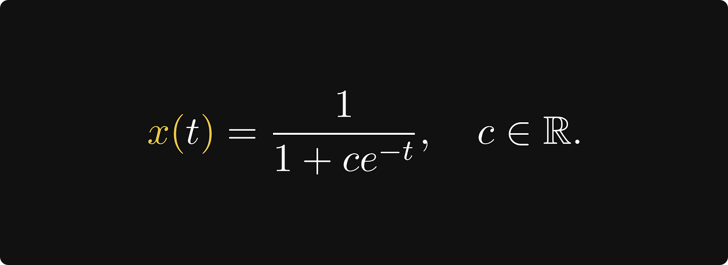
With a little bit of calculation (whose details are not essential for us), we can obtain that the solutions are
(c is an arbitrary constant.) For c = 1, this is the famous Sigmoid function. You can check by hand that these are indeed solutions. We can even plot them, as shown below.
As we can see, the monotonicity of the solutions is as we predicted.
We can characterize the equilibria based on the long-term behavior of nearby solutions. (In the case of our logistic equation, the equilibria are 0 and 1.) This can be connected to the local behavior of f: if it decreases around the equilibrium x*, it attracts the nearby solutions. On the other hand, if f increases around x*, the nearby solutions are repelled.
This gives rise to the concept of stable and unstable equilibria.
In the case of the logistic ODE x′ = x(1−x), x* = 1 is a stable and x* = 0 is an unstable equilibrium. This makes sense given its population dynamics interpretation: the equilibrium x* = 1 means that the population is at maximum capacity. If the size is slightly above or below the capacity 1, some specimens die due to starvation, or the colony reaches its constraints. On the other hand, no matter how small the population is, it won't ever go extinct in this ideal model.
A continuous version of gradient ascent
Now, let's talk about maximizing the real function F. Suppose that F is twice differentiable, and we denote its derivative by F′ = f. Luckily, the local maxima of F can be found with the help of its second derivative by looking for x* where f(x*) = 0 and
f ′(x*) < 0.
Does this look familiar? If f(x*) = 0 indeed holds, then x(t) = x* is an equilibrium solution; and since f ′(x*) < 0, it attracts the nearby solutions as well. This means that if x₀ is drawn from the basin of attraction and x(t) is the solution of the usual initial value problem, then the solution converges towards x*, a local maxima of F! This is gradient ascent in a continuous version.
We are happy, but there is an issue. We've talked about how hard solving differential equations are. For a general F, we have no prospects to actually find the solutions. Fortunately, we can approximate them.
Gradient ascent as a discretized differential equation
When doing differentiation in practice, derivatives are often approximated numerically by the forward difference
If x(t) is indeed the solution for the corresponding initial value problem, we are in luck! Using forward differences, we can take a small step from 0 and approximate x(h) by substituting the forward difference into the differential equation. To be precise, we have
from which
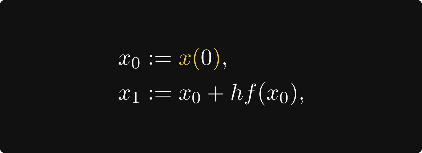
follows. By defining x₀ and x₁ by
we have x₁ ≈ x(h). If this looks like the first step of the gradient ascent to you, you are on the right track. Using the forward difference once again, this time from the point x(h), we obtain
thus by defining x₂ := x₁+hf(x₁), we have x₂ ≈ x(2h). Notice that in x₂, two kinds of approximation errors are accumulated: first the forward difference, then the approximation error of the previous step.
This motivates us to define the recursive sequence
which approximates x(nh) with xₙ, as this is implied by the very definition. This recursive sequence is the gradient ascent itself, and the small step h is the learning rate! In the context of differential equations, this is called the Euler method.
Without going into the details, if h is small enough and f "behaves properly", the Euler method will converge to the equilibrium solution x*. (Whatever proper behavior might mean.)
We only have one more step: to turn everything into gradient descent instead of ascent. This is extremely simple, as gradient descent is just applying gradient ascent to −f. Think about it: minimizing f is the same as maximizing −f. And with that, we are done! The famous gradient descent is a consequence of dynamical systems converging towards their stable equilibria, and this is beautiful.
The gradient ascent in action
To see the gradient ascent (that is, the Euler method) in action, we should go back to our good old example: the logistic equation
So, suppose that we want to find the local maxima of the function
which is plotted below.
First, we can use what we learned and find the maxima using the derivative, concluding that there is a local maximum at x* = 1. (Don't just take my word, pick up a pencil and work it out!)
Since f(x*) = F′(x*) = 0 and f ′(x*) < 0, the point x* is a stable equilibrium of the logistic equation. Thus, if the initial value x(0) = x₀ is sufficiently close to x* = 1, the solution of the initial value problem will converge to x*.
(In fact, we can select any initial value from the infinite interval (0,∞), and the convergence will hold.) Upon discretization via the Euler method, we obtain the recursive sequence
This process is visualized below, where the solutions of the logistic equation via the Euler method are plotted. Smaller h gives a better approximation.
We can even take the discrete solution provided by the Euler method and plot it on the x-F(x) plane.
Conclusion
To sum up what we've seen so far, our entire goal was to understand the very principles of gradient descent, the most important optimization algorithm in machine learning. Its main principle is straightforward: to find a local minimum of a function, first find the direction of decrease, then take a small step towards there. This seemingly naive algorithm has a foundation that lies deep within differential equations. Turns out that if we look at our functions as rules determining a dynamical system, local extrema correspond to equilibrium states. These dynamical systems are described by differential equations, and the local maxima of our function are equilibrium states that attracts solutions towards them. From this viewpoint, the gradient descent algorithm is nothing else than a numerical solution to this equation.
What we've seen so far only covers the single-variable case, and as I have probably told this many times, machine learning is done in millions of dimensions. Still, the intuition we built up will be our guide in the study of multivariable functions and high-dimensional spaces. There, the principles are the same, but the objects of study are much more complex. The main challenge in multivariable calculus is to manage the complexity, and this is where our good friends, vectors and matrices will do much of the heavy lifting. But that's for another day!
If you are interested what’s behind machine learning techniques such as this, check out my Mathematics of Machine Learning book! The early access is out, and new chapters are added as I write them.












Well explained 💯🔥
I like the differential equations view. People tend to add a disclaimed that it's the "small step size limit", but turns out this approximation works quite well even for large step size in high dimensions. Step size is bounded by largest eigenvalue, but if most of the mass comes from remaining dimensions, the "large" step size is actually quite small. I did some visualizations on this a while back https://machine-learning-etc.ghost.io/gradient-descent-linear-update/