
What's the meaning of the expected value?
An intuitive explanation

I was using the concept of expected value long before I understood anything about probability theory.
Back in high school, I was a fan of no limit Texas hold’em, and I quickly learned the concept of pot odds. Say, if I would win the hand with 10 cards and would lose with the remaining 40, I should only call a bet if it is not larger than the quarter of the current pot.
This is called positive pot odds.

Why should you only play with positive pot odds? Because on the long run, such calls are profitable; others are not.
Fast forward a few years. Instead of playing poker, I am sitting in my introductory probability theory class as a math major, and the teacher explains us the expected value.

Suddenly, it all made sense: pot odds are expected value, and it is one of the single most useful concepts in probability theory and statistics.
However, this is not immediately obvious by the mathematical formula.
How did this story about pot odds come to my mind? Because I am writing a chapter exactly about the expected value for my Mathematics of Machine Learning book. I am looking for ways to clearly explain the meaning behind these not-so-intuitive formulas, and I think I came up with something worth sharing.
So, here is the story of expected value.
A simple game of chance
Let’s put poker aside for now, and play an even simpler game.
The rules are straightforward. I’ll toss a coin, and if it comes up heads, you win $1. However, if it is tails, you lose $2.
Should you even play this game with me? We’ll find out.
After n rounds, your earnings can be calculated by the number of heads times $1 minus the number of tails times $2. If we divide total earnings by n, we obtain your average earnings per round.

What happens when n approaches infinity?
As you have probably guessed, the number of heads divided by the number of tosses will converge to the probability of a single toss being heads.
Similarly, tails per tosses also converge to 1/2.

With this in mind, we can explicitly calculate your average earnings per round.
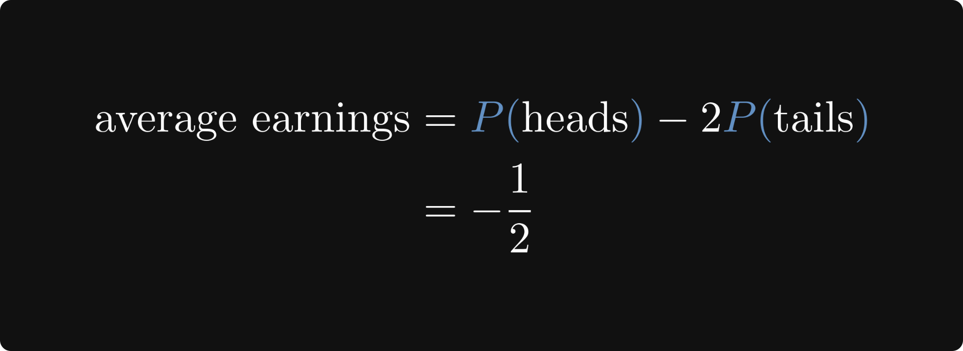
Your average earnings are -1/2 per round. So, you definitely shouldn't play this game.
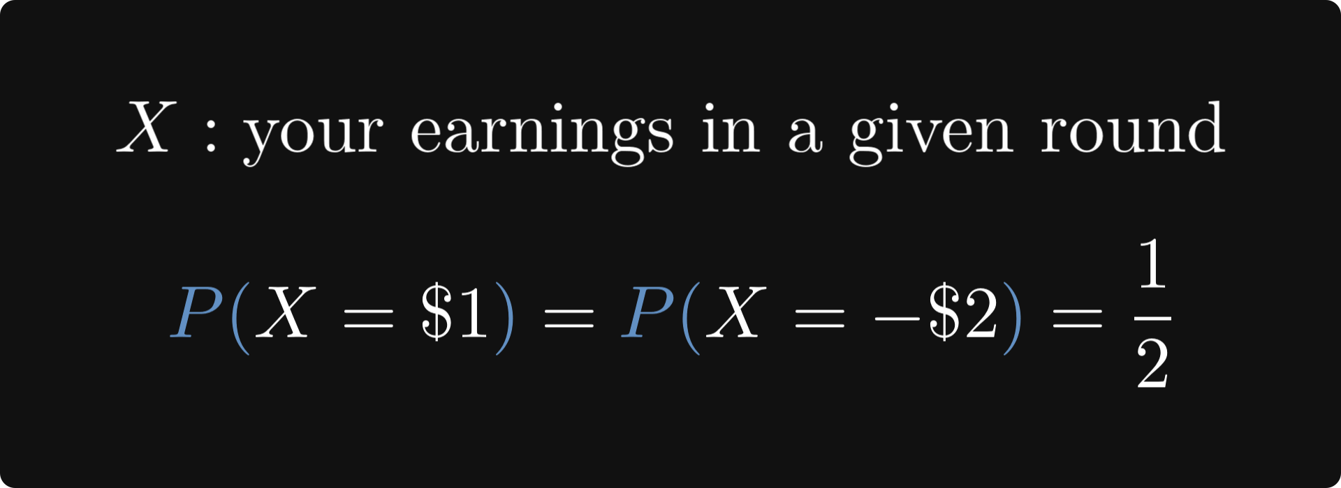
This is the expected value! To see this, let’s formalize our little game with a random variable X, denoting your earnings.
By plugging this into the formula of expected value, we obtain just what we calculated before: the average earnings per round!
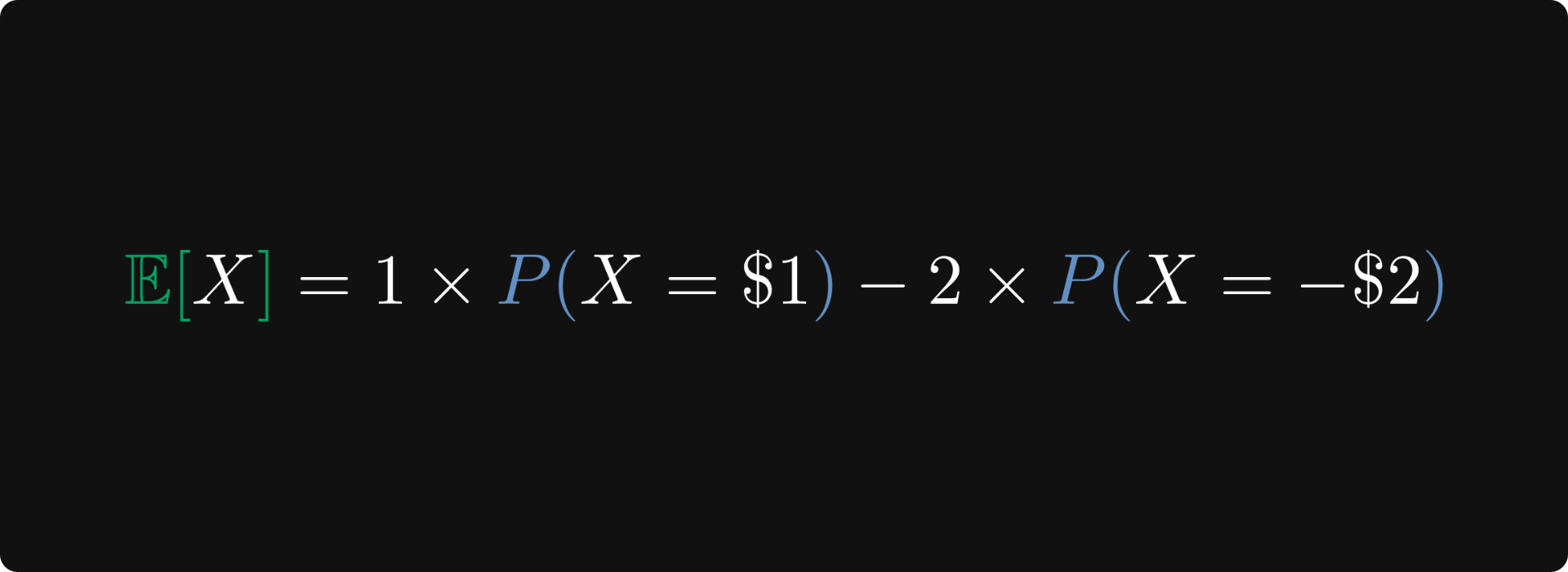
In plain English, the expected value is just the average outcome per experiment when you let it run infinitely!

To sum up, let’s look at the general formula. In essence, the expected value is the average of all possible outcomes, weighted by their respected probabilities.

Awesome! Let’s see another example, the one mentioned in the introduction.
Pot odds in poker
Do you recall the pot odds formula? Here it is below.

What does this have to do with the expected value? I’ll explain.
According to the rules of Texas hold-em, each player holds two cards on their own, while five more shared cards are dealt. The shared cards are available for everyone, and the player with the strongest hand wins.
This is how the table looks before the last card (the river) is revealed.

There is money in the pot to be won, but to see the river, you have to call the opponent’s bet.
The question is, should you? Expected value to the rescue.
Let’s build a probabilistic model. We would win the pot with certain river cards (the good ones), but lose with all the others (the bad ones).

The rule is simple: if the expected winnings are positive, we call the bet. Otherwise, we fold.
We can quantify this using the expected value.

With some algebra, we obtain that our expected winnings are positive if the ratio of good and bad cards is better than the ratio of the bet and the pot.

Of course, this is extremely hard to determine in practice. For instance, you don’t know what others hold, and counting the cards that would win the pot for you is not possible unless you have a good read on the opponents. So, it’s much more than just math. Good players choose their bet specifically to throw off their opponents pot odds.
Is this everything about the expected value?
No. What about experiments where the set of possible outcomes is not countable? Can we apply the same thinking?
Let’s find out.
Continuous random variables
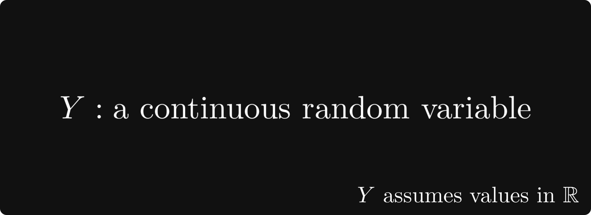
In practice, not all experiments can be described with discrete outcomes. For instance, the random variable encoding the lifespan of a lightbulb can assume any real number.
From now on, assume that Y is a continuous random variable; that is, real-valued with an existing density function.
What happened in the discrete case?
We can visualize a discrete random variable via its mass distribution: at each potential outcome, a bar with its height matching the probability stands.

The interpretation of the expected value was simple: outcome times probability, summed over all potential values.
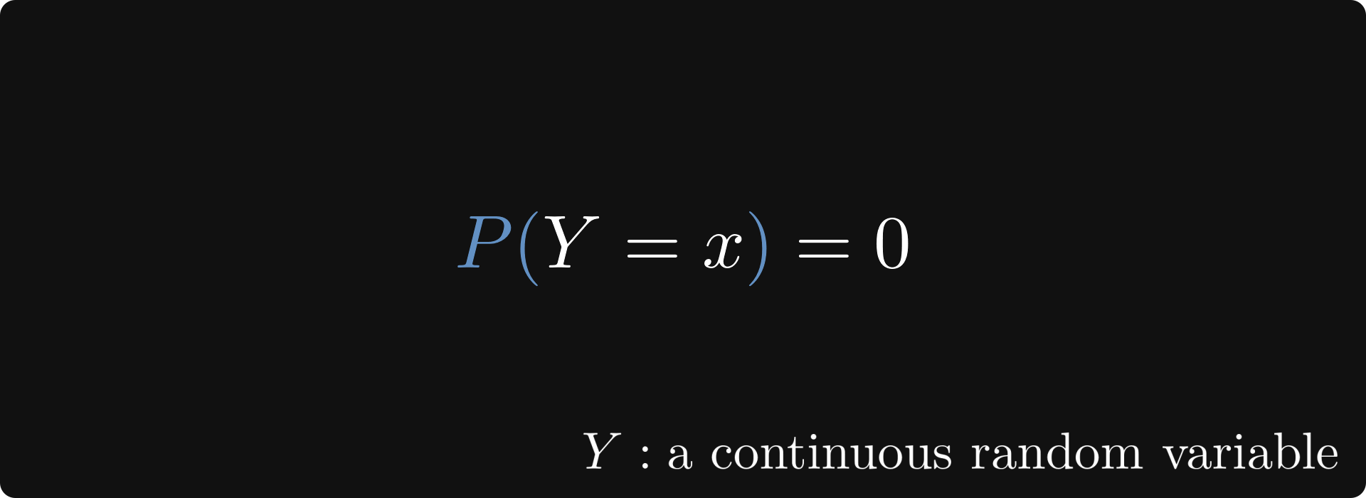
However, there is a snag with continuous random variables: we don’t have such a mass distribution, as the probabilities of individual outcomes are zero.
What can we do?
Wishful thinking. This is one of the most powerful techniques in mathematics, and I am not joking.
Here’s the plan. We’ll pretend that the expected value of a continuous random variable is well-defined, and let our imagination run free. Say goodbye to mathematical precision, and allow our intuition to unfold.
Instead of the probability of a given outcome, we can talk about X landing in a small interval. First, we divide up the set of real numbers into really small parts, delimited by the values xₖ.
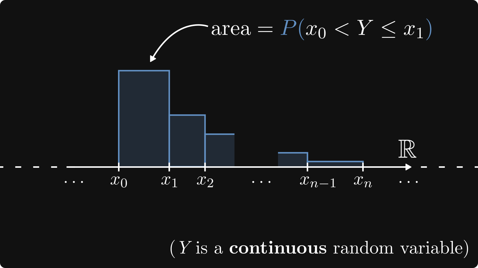
This can be represented by a properly defined histogram. Just like a smoothed version of a discrete mass distribution.
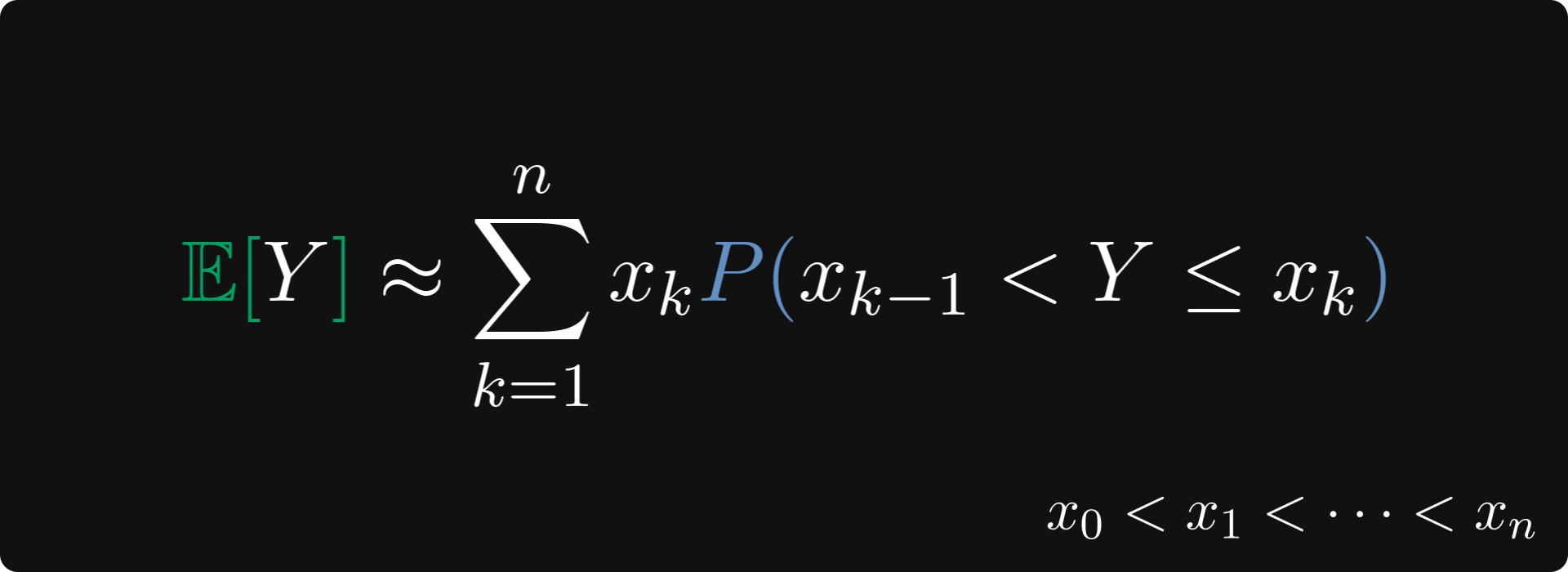
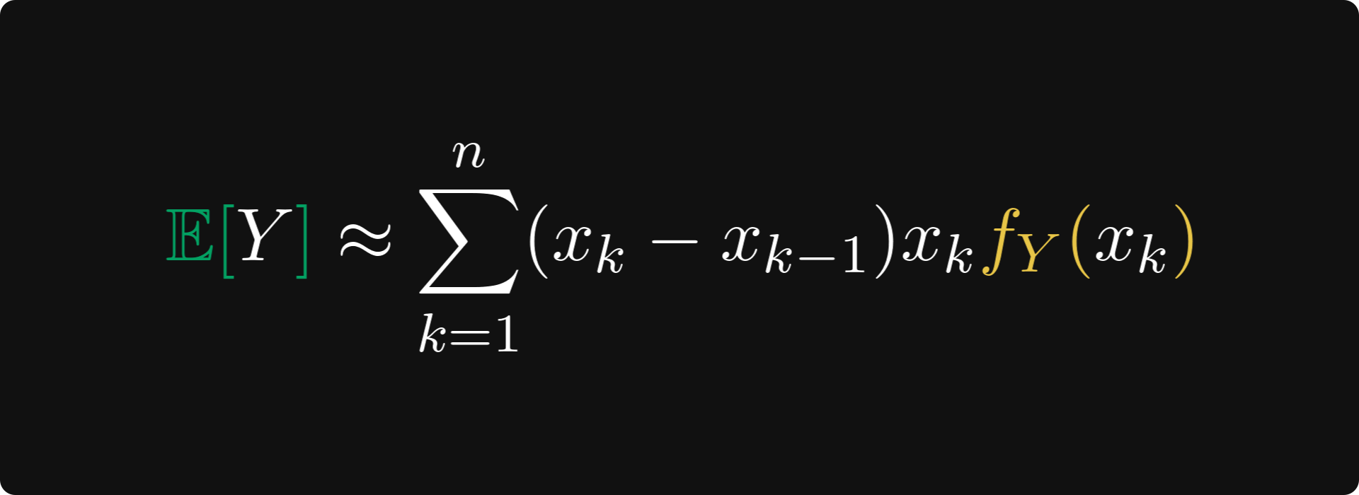
By applying the “average outcome = sum of outcome x probability“ logic, the expected value should be close to this value below. (At least if the intervals are small enough, and cover the range of Y fairly well.)
What now?
With a move similar to pulling out a rabbit from the magician’s hat, we can notice that by scaling the probabilities with the interval’s length, our intuition can go one step further.
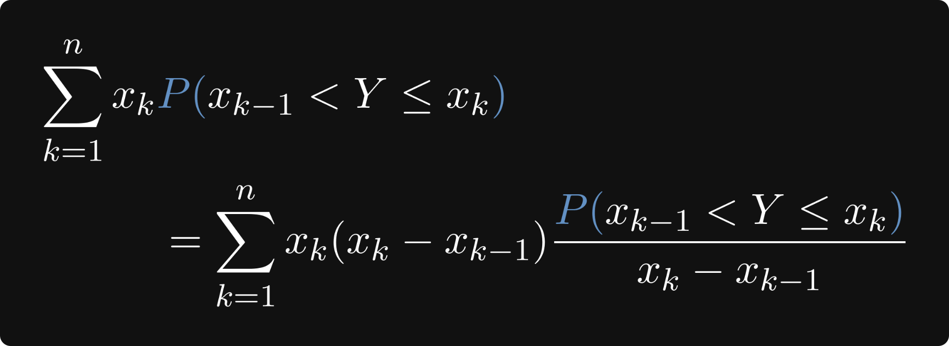
Why? Because this probability can be expressed with the cumulative distribution function (or CDF in short) of Y.

In turn, if the intervals are small enough, the resulting difference quotients are close to the density function, which is the derivative of the CDF.

Again, nothing is mathematically precise here, we are just working with our intuition.
The result: if the expected value does indeed exist, it should be close to the sum below.
This was our goal the entire time. Why?
Because this is (almost) a Riemann-sum, approximating the integral of the function inside. At least, this is what our intuition suggests.
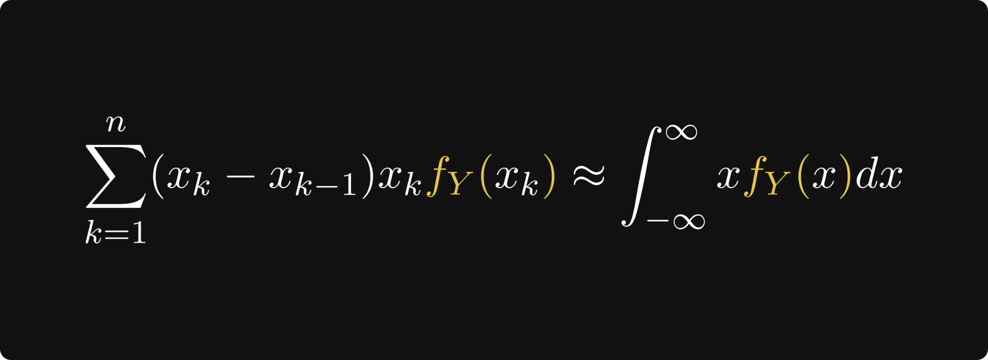
We have arrived at the finish line. We started from the “average outcome = sum of outcome x probability“ formula and ended up with the integral of x times the density function.
The result is completely analogous to the discrete case, but instead of probabilities, we have a density.

Our argument leading to the integral formula can be made precise with some mathematical heavy machinery, but trust me on this, the intuition behind is far more interesting. (At least, for non-mathematicians.)
Conclusion
Overall, the expected value is one of the most important concepts of probabilistic thinking.
It’s not just for determining whether or not we should call bets: it’s the cornerstone of statistics and machine learning. For instance, the mean squared error, entropy, and Kullback-Leibler divergence are all expected values.
The most important part: for both discrete and continuous random variables, the expected value represents the average outcome.

What I told you here is just the tip of the iceberg. If you have liked this explanation, check out my Mathematics of Machine Learning early access book! There’s much more there.
Currently, I am working on the probability theory and statistics chapter with full force. I release each chapter as I write them, and the one about the expected value should come soon.
Great post. I love them!
Hint: consider the repeated product of the returns. This is also a good motivator for talking about kl divergence / Jensen's inequality