


The Roadmap of Mathematics for Machine Learning
A complete guide to linear algebra, calculus, and probability theory

Understanding the mathematics behind machine learning algorithms is a superpower.
If you have ever worked on a real-life problem, you probably experienced that being familiar with the details can go a long way if you want to move beyond baseline performance. This is especially true when you want to push the boundaries of state-of-the-art.
However, most of this knowledge is hidden behind layers of advanced mathematics. Understanding methods like stochastic gradient descent may seem difficult, as they are built on top of multivariable calculus and probability theory.
With proper foundations, though, most ideas can be seen as quite natural. If you are a beginner and don’t necessarily have formal education in higher mathematics, creating a curriculum for yourself is hard. In this post, my goal is to present a roadmap that takes you from absolute zero to a deep understanding of how neural networks work.
To keep things simple, the aim is not to cover everything. Instead, we will focus on getting our directions. This way, you will be able to study other topics without difficulties, if need be.
Instead of reading through in one sitting, I recommend using this article as a reference point through your studies. Go deep into a concept that is introduced, then check the roadmap and move on. I firmly believe that this is the best way to study: I will show you the road, but you must walk it.
Machine learning is built upon three pillars: linear algebra, calculus, and probability theory.
Here’s the full roadmap for you.
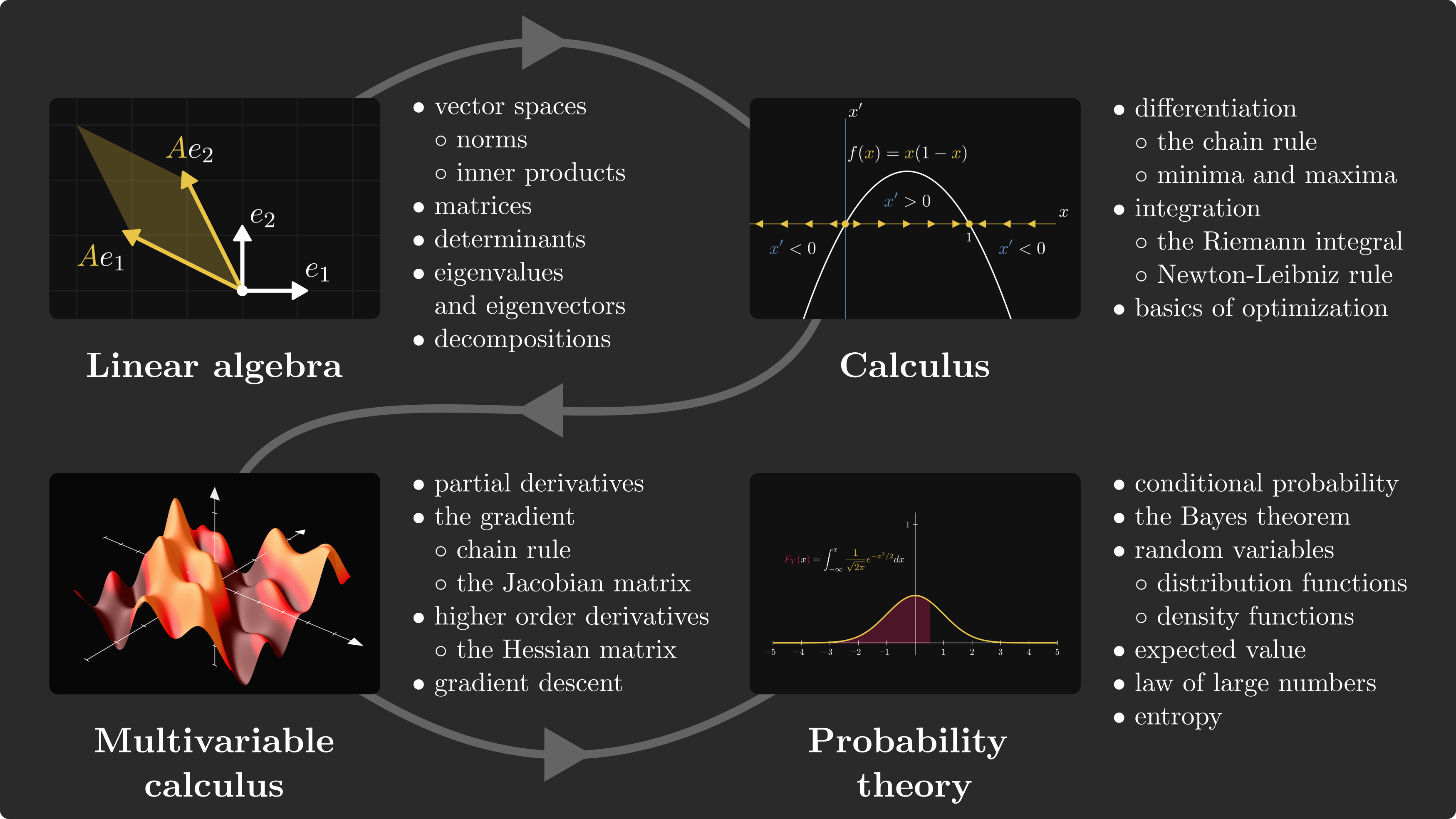
Linear algebra is used to describe models, calculus is to fit the model to the data, and probability theory is to tie it all together by providing a theoretical framework for making predictions under uncertainty.
What follows is a ~4000 words-long deep dive into all of these, where we’ll walk through the main topics step by step.
If you are interested in the mathematics of machine learning, this is the article you want to read.
📌 The Palindrome breaks down advanced math and machine learning concepts with visuals that make everything click.
Join the premium tier to get instant access to guided tracks on graph theory, foundations of mathematics, and neural networks from scratch.
A quick note. This post is way to long for email. For the best experience, read the post in your browser or in the Substack app.
Linear algebra
Predictive models such as neural networks are essentially functions that are trained using the tools of calculus. However, they are described using linear algebraic concepts, such as matrix multiplication.
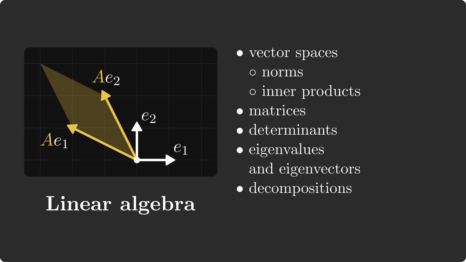
If you are a machine learning engineer working on real-life problems, linear algebra is the most important topic for you, and mastering it will put you above the playing field.
Let’s dive deep!
Vectors and vector spaces
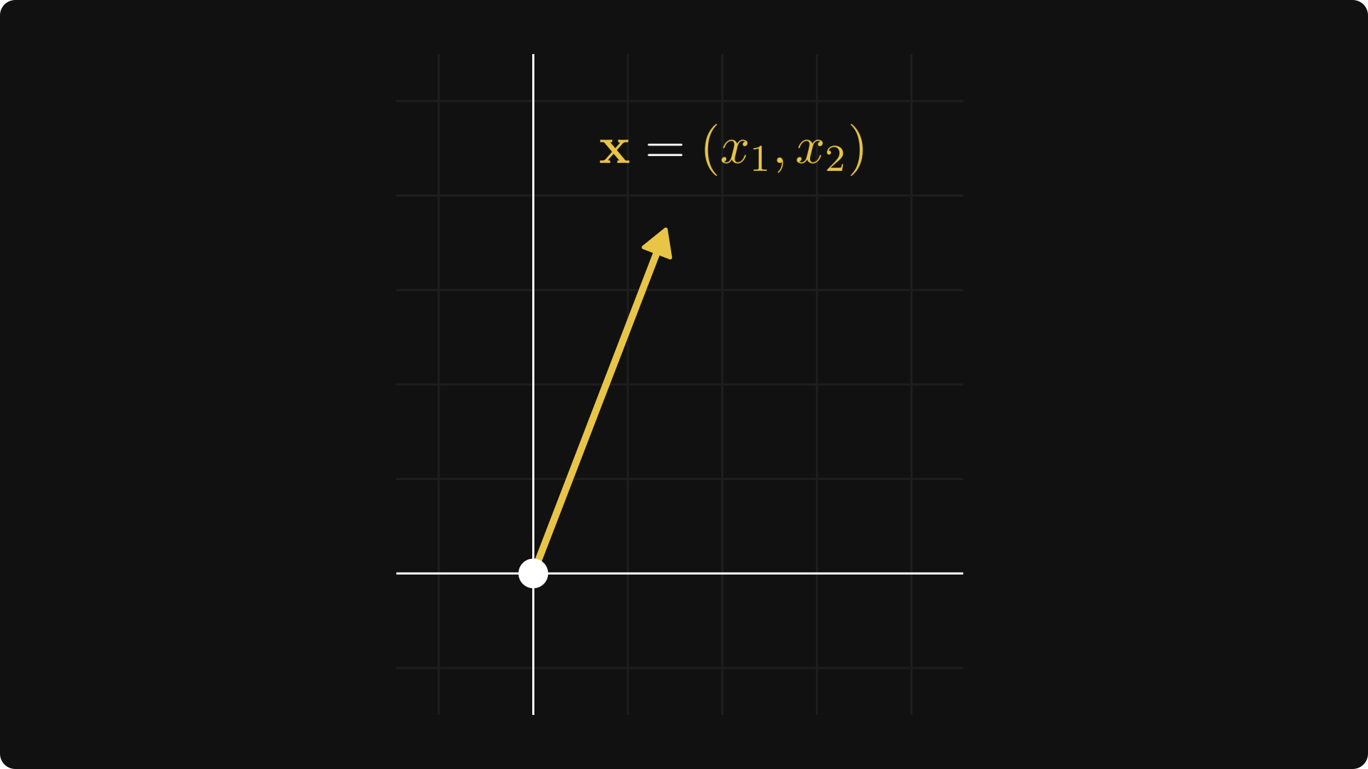
To have a good understanding of linear algebra, I suggest starting with vector spaces.
The textbook definition is intimidating and abstract, so let’s talk about a special case first. You can think of each point in the plane as a tuple x = (x₁, x₂), represented by an arrow pointing from the origin to (x₁, x₂).
You can add these vectors together and multiply them with scalars. Algebraically, it simply goes as
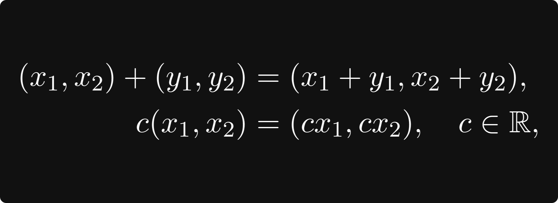
but it’s easier to visualize:
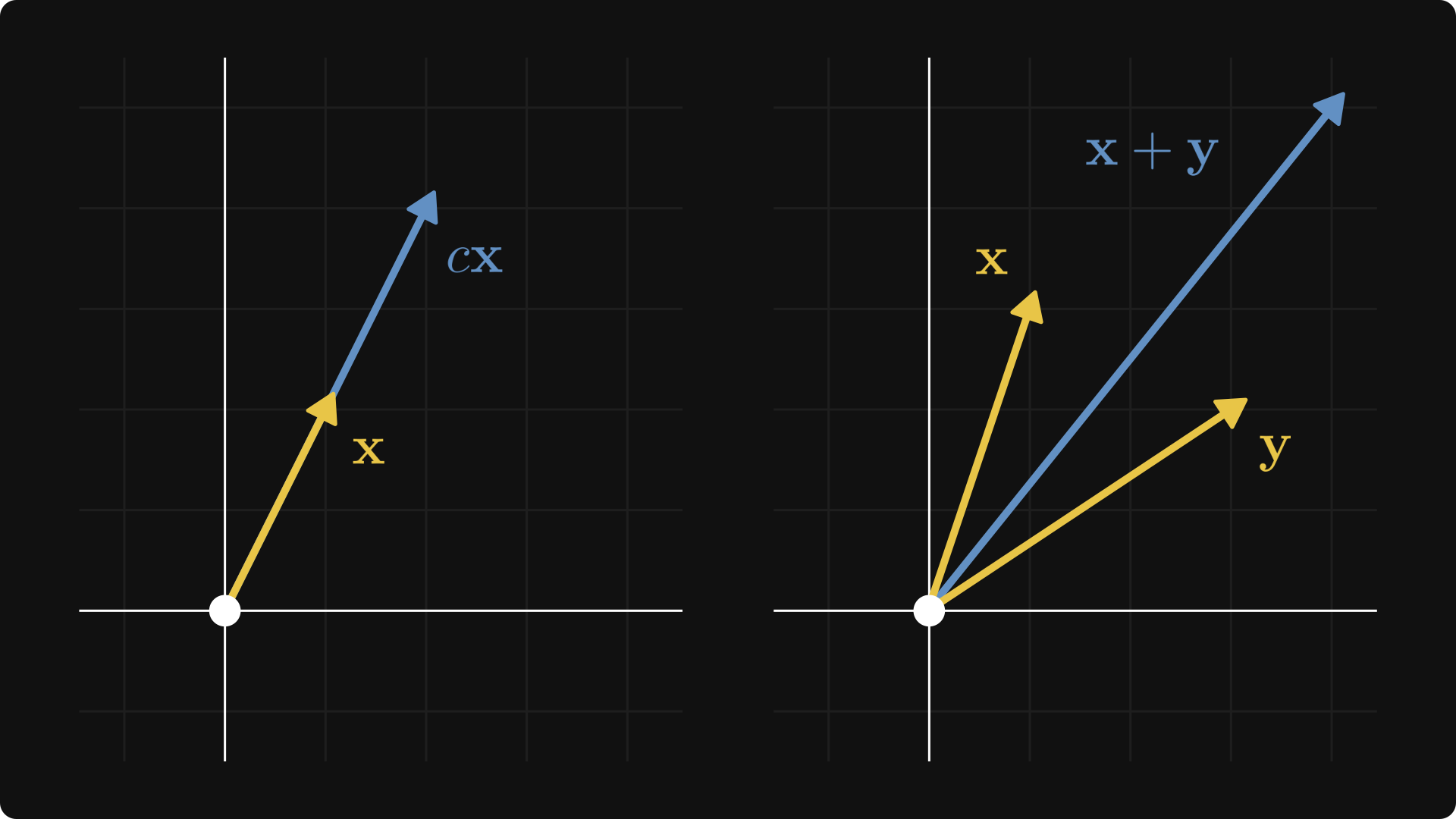
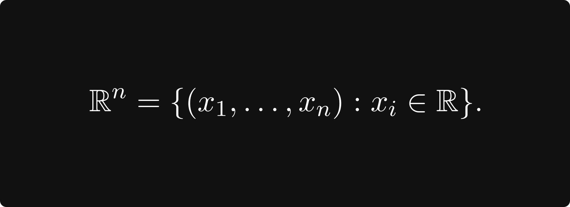
The Euclidean plane is the prototypical model of a vector space. Tuples of n elements form n-dimensional vectors, making up the Euclidean space
In general, a set of vectors V is a vector space over the real numbers if you can add and scale vectors in a straightforward way.
When thinking about vector spaces, it helps to model them as tuples in Euclidean space mentally.
Normed spaces
When you have a good understanding of vector spaces, the next step is to understand how to measure distance in vector spaces.
By default, a vector space in itself gives no tools for this. How would you do this on the plane? You have probably learned that there, we have the famous Euclidean norm defined by
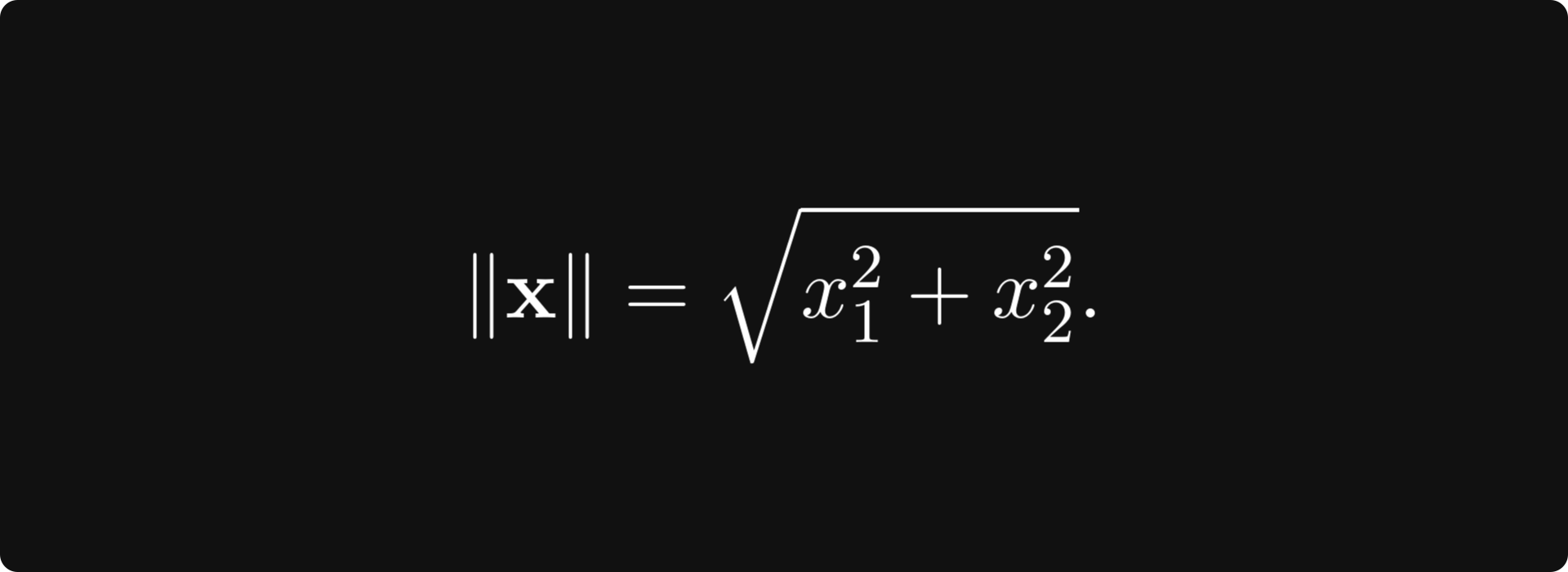
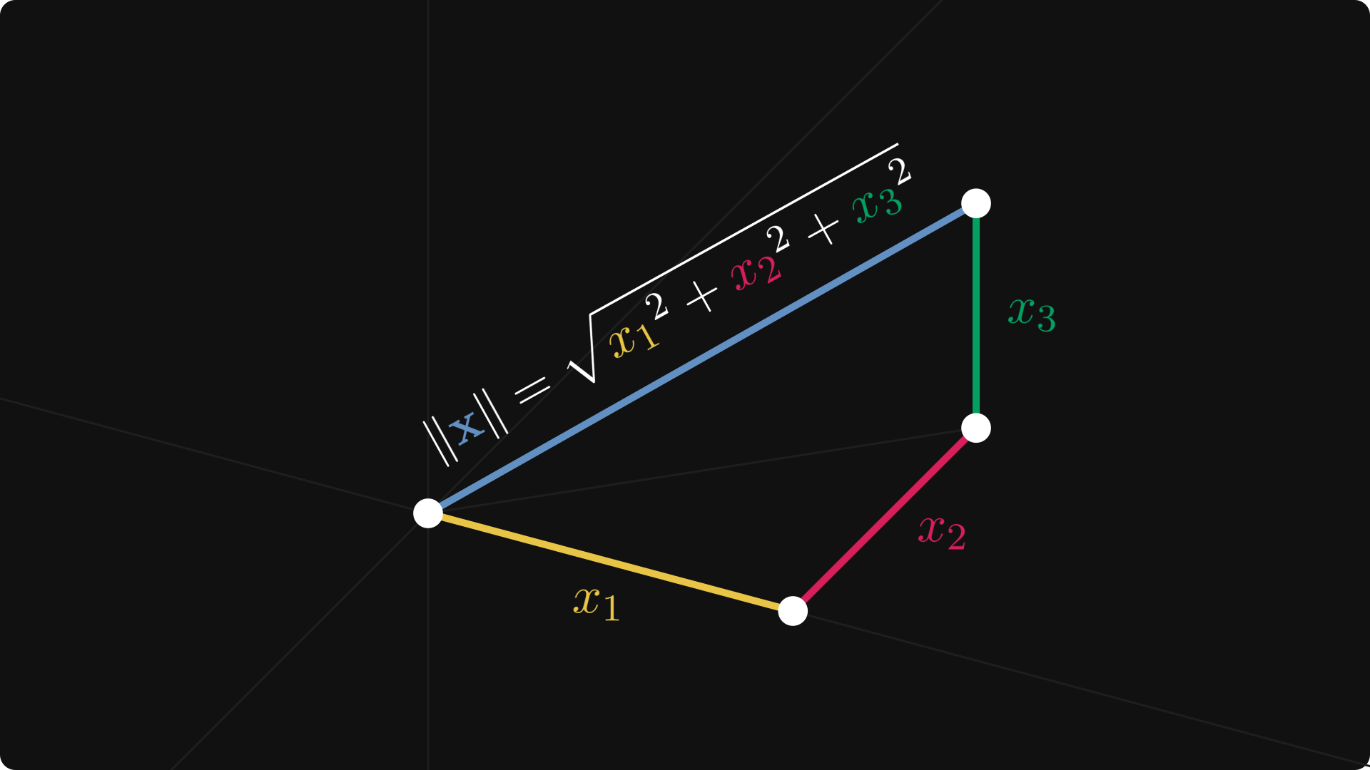
Although the vector notation and the square root symbol make this feel intimidating, the magnitude is just the Pythagorean theorem in disguise.
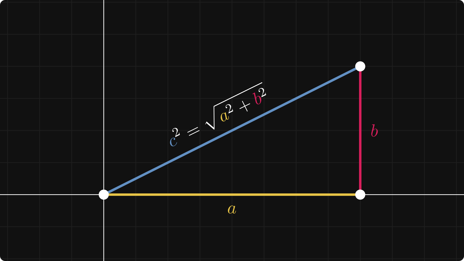
This can be generalized further: in three dimensions, the Euclidean norm is the repeated application of the Pythagorean theorem.
This is a special case of a norm. In general, a vector space V is normed if there is a function ‖ ⋅ ‖: V → [0, ∞) such that
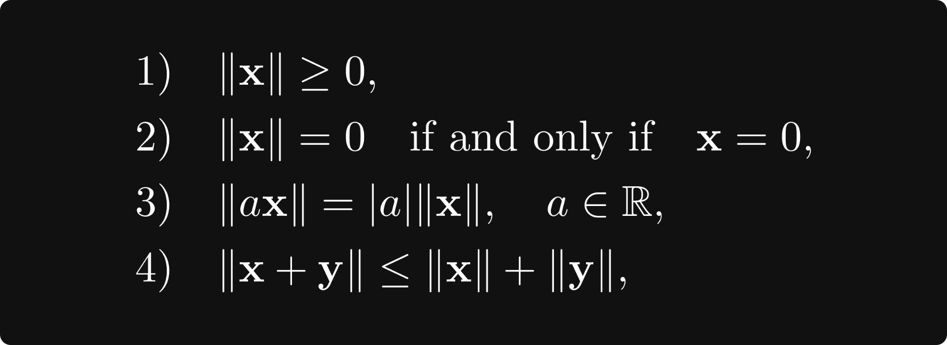
where x and y are any two vectors.
Again, this might be scary, but this is a simple and essential concept. There are a bunch of norms out there, and the most important is the p-norm family, defined for any p ∈ [0, ∞) by
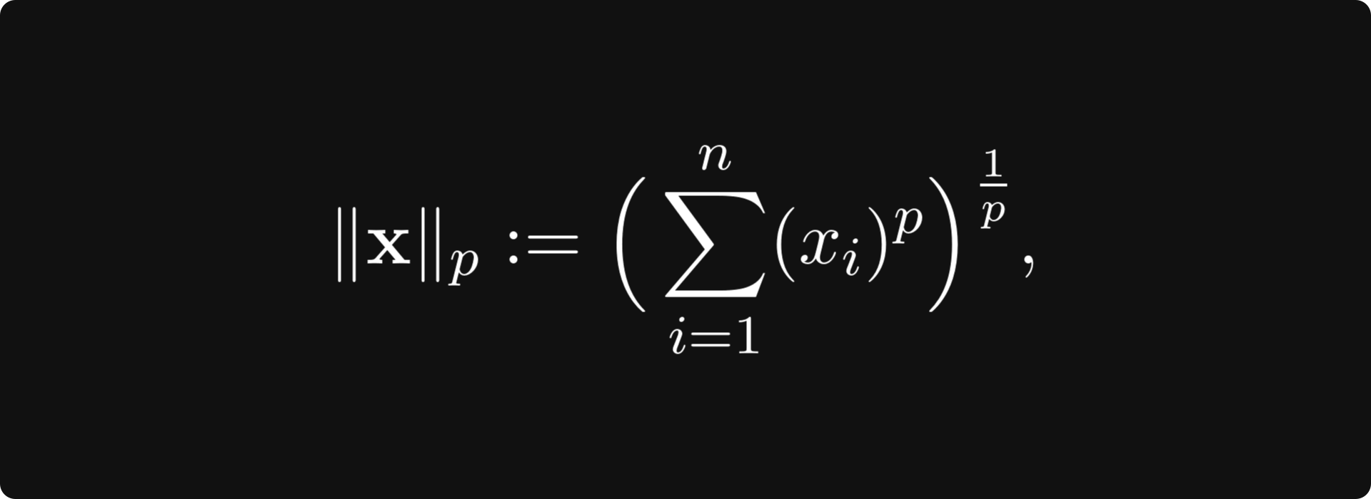
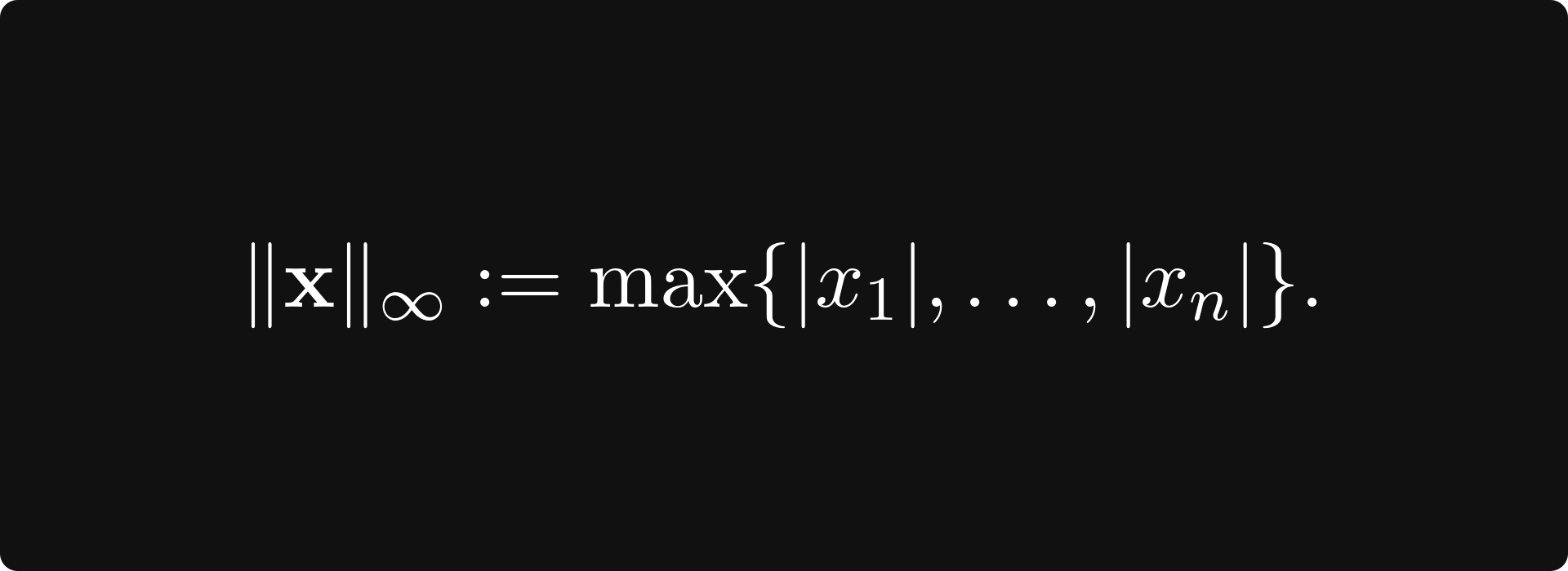
(with p = 2 giving the Euclidean norm) and the supremum norm
Norms can be used to define a distance by taking the norm of the difference:
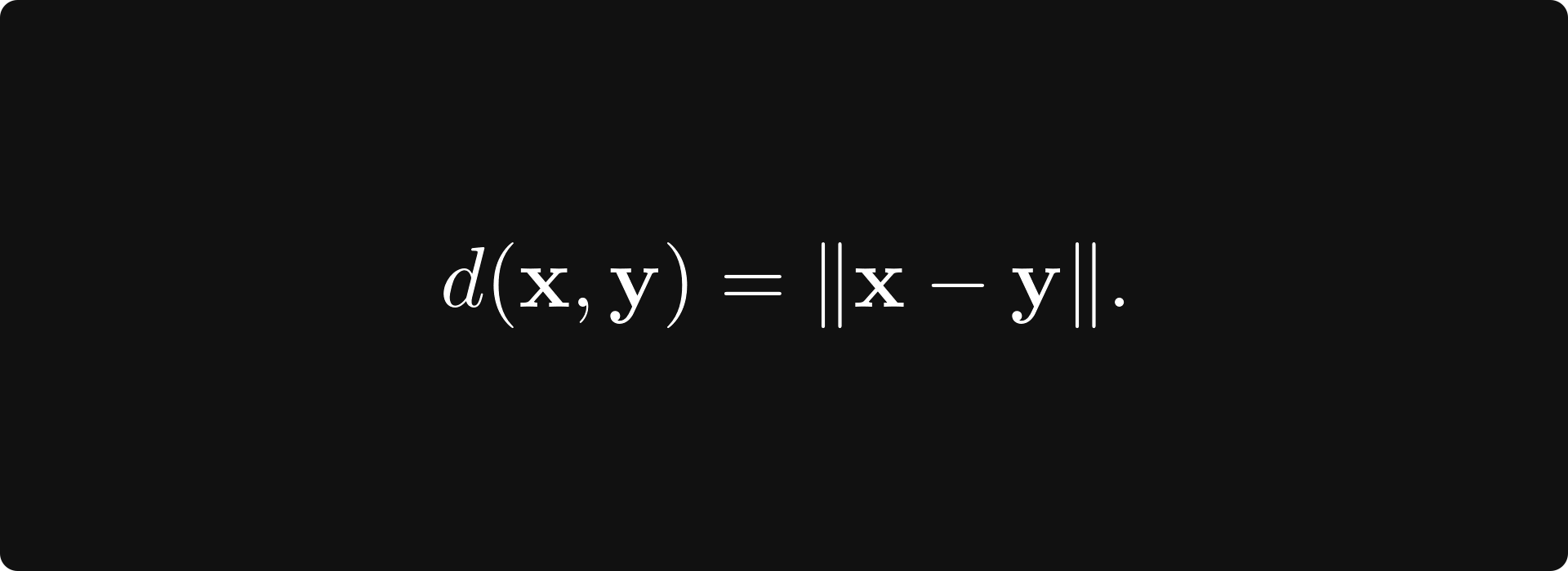
The 1-norm is called the Manhattan norm (or taxicab norm), because the distance between two points depends on how many “grid jumps” you have to perform to get from x to y.

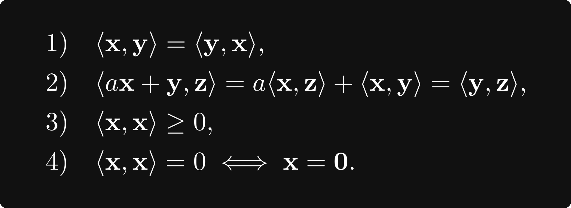
Sometimes, like for p = 2, the norm comes from a so-called inner product, which is a bilinear function 〈 ⋅, ⋅ 〉: V × V → [0, ∞) such that
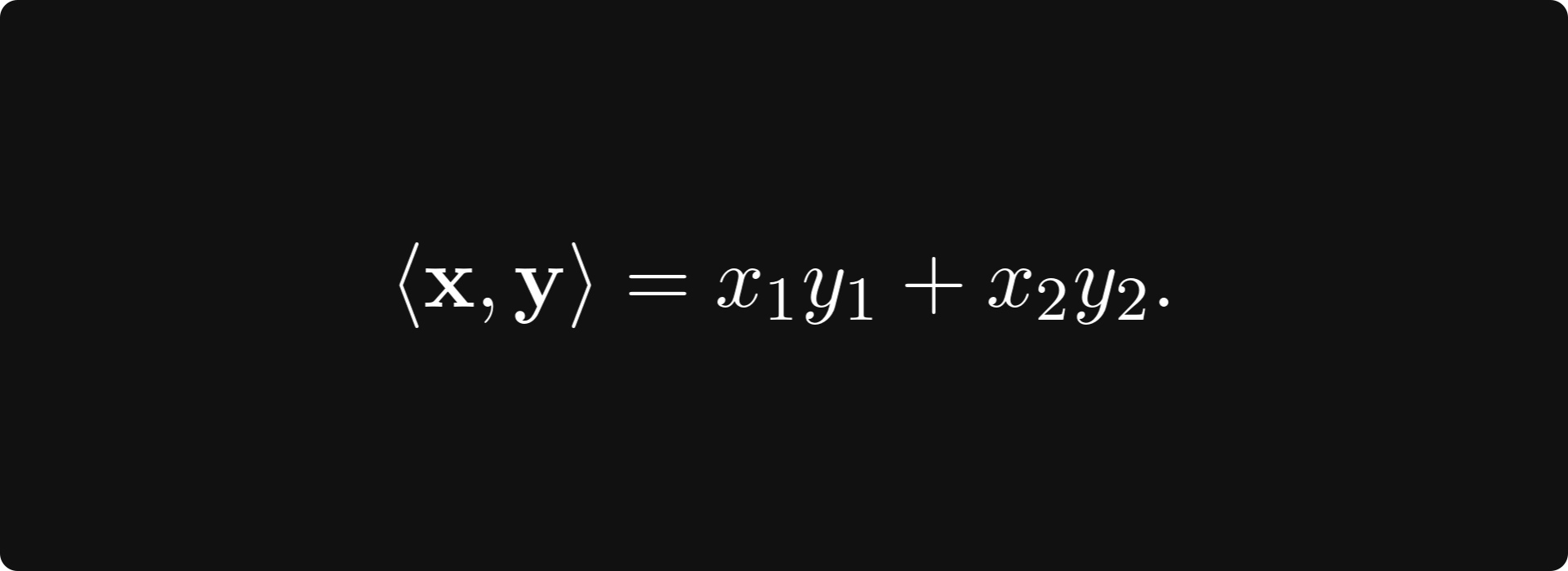
A vector space with an inner product is called an inner product space. An example is the classical Euclidean product
On the other hand, every inner product can be turned into a norm by

When the inner product for two vectors is zero, we say that the vectors are orthogonal to each other. (Try to come up with some concrete examples on the plane to understand the concept more deeply.)
Basis and orthogonal/orthonormal basis
Although vector spaces are infinite (in our case), you can find a finite set of vectors that can be used to express all vectors in the space. For example, on the plane, we have
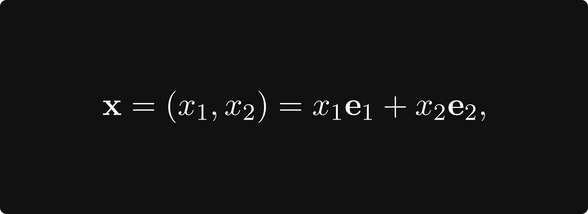
where

This is a special case of a basis and an orthonormal basis.
In general, a basis is a minimal set of vectors v₁, v₂, ..., vₙ ∈ V such that their linear combinations span the vector space:
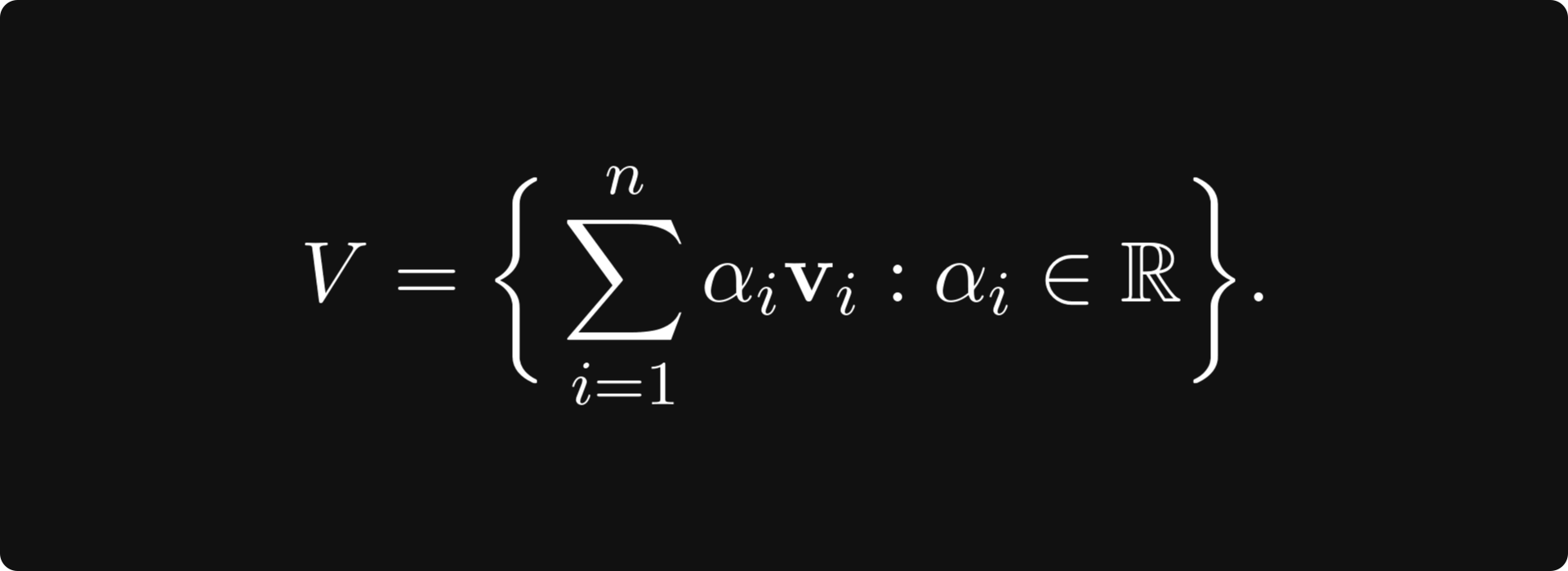
A basis always exists for any vector space. (It may not be a finite set, but that shouldn’t concern us now.) Without a doubt, a basis simplifies things greatly when talking about linear spaces.
When the vectors in a basis are orthogonal to each other, we call it an orthogonal basis. If each basis vector’s norm is 1 for an orthogonal basis, we say it is orthonormal.
Linear transformations
The key objects related to vector spaces are linear transformations. If you have seen a neural network before, you know that the fundamental building blocks are layers of the form f(x) = σ(Ax + b), where A is a matrix, b and x are vectors, and σ is the sigmoid function. (Or any activation function, really.) Well, the part Ax is a linear transformation.
In general, the function L: V → W is a linear transformation between vector spaces V and W if
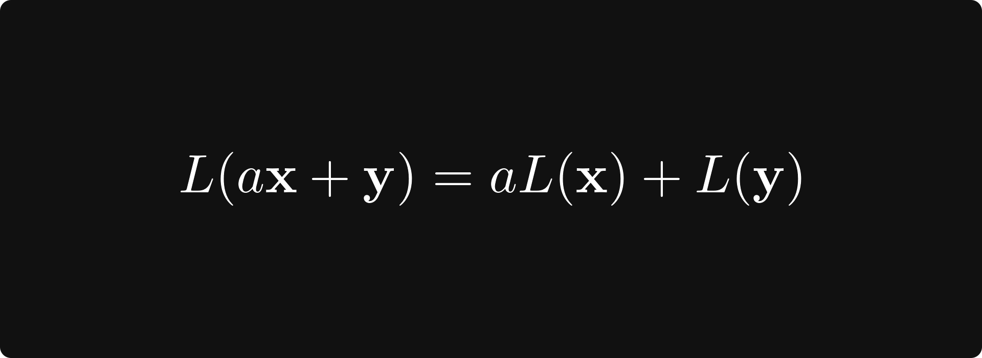
holds for all x, y in V, and all real number a.
To give a concrete example, rotations around the origin in the plane are linear transformations.
Undoubtedly, the most crucial fact about linear transformations is that they can be represented with matrices, as you’ll see next in your studies.
Matrices and their operations
If linear transformations are clear, you can turn to the study of matrices. (Linear algebra courses often start with matrices, but I would recommend it this way for reasons to be explained later.)
The most important operation for matrices is matrix multiplication, also known as the matrix product. In general, if A and B are matrices defined by
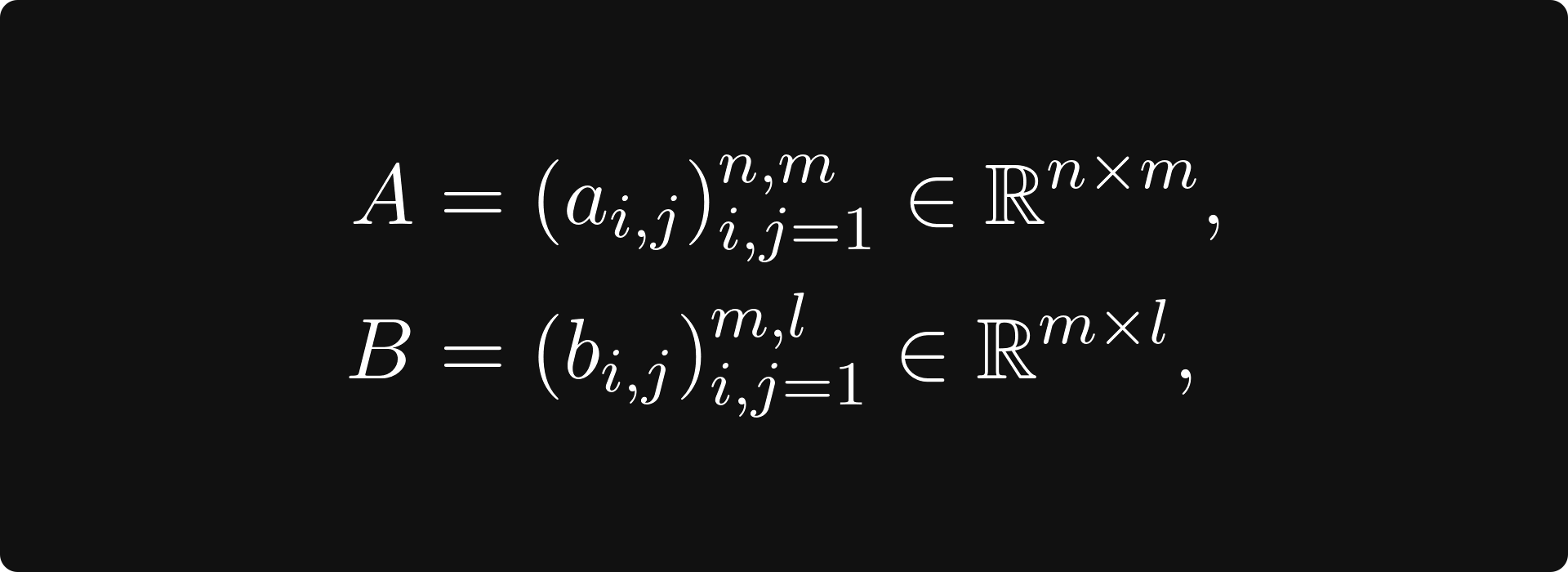
then their product can be obtained by
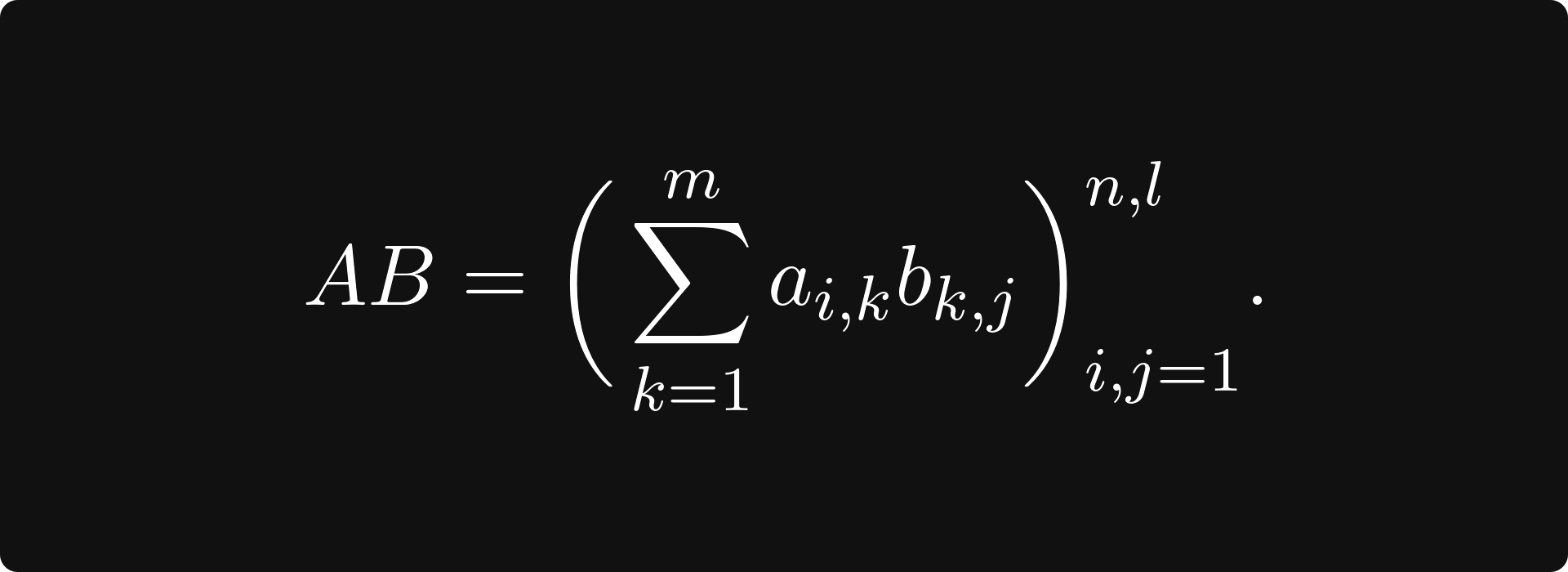
This might seem difficult to comprehend, but it is pretty straightforward. Take a look at the figure below, demonstrating how to calculate the element in the 2nd row, 1st column of the product.
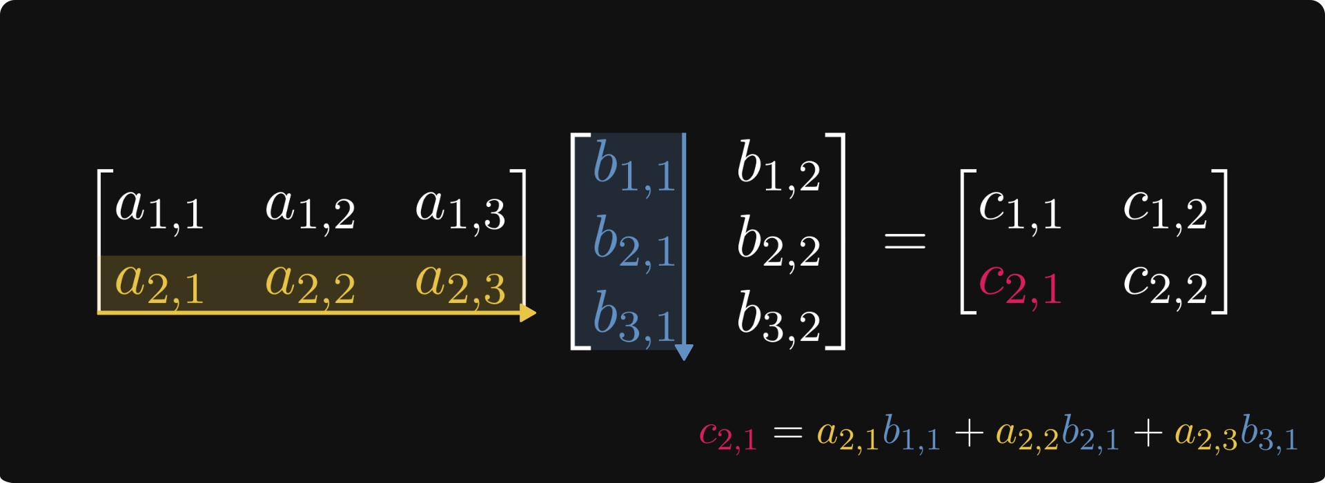
The reason why matrix multiplication is defined the way it is because matrices represent linear transformations between vector spaces. Matrix multiplication is the composition of linear transformations.
Determinants
In my opinion, determinants are hands down one of the most challenging concepts to grasp in linear algebra. Depending on your learning resource, it is usually defined by either a recursive definition or a sum that iterates through all permutations. None of them is tractable without significant experience in mathematics.
To understand this concept, watch this video below. Trust me, it is magic.
To summarize, the determinant of a matrix describes how the volume of an object scales under the corresponding linear transformation. If the transformation changes orientations, the sign of the determinant is negative.
You will eventually need to understand how to calculate the determinant, but I wouldn’t worry about it now.
Eigenvalues, eigenvectors, and matrix decompositions
A standard first linear algebra course usually ends with eigenvalues/eigenvectors and some special matrix decompositions like the Singular Value Decomposition.
Let’s suppose that we have a matrix A. The number λ is an eigenvalue of A if there is a vector x (called an eigenvector) such that Ax = λx holds. In other words, the linear transformation represented by A is a scaling by λ for the vector x. This concept plays an essential role in linear algebra. (And practically in every field that uses linear algebra extensively.)
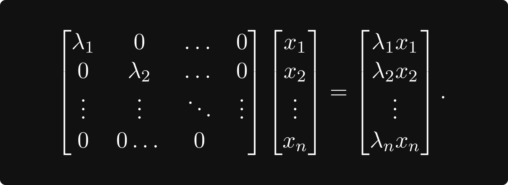
At this point, you are ready to familiarize yourself with a few matrix decompositions. If you think about it for a second, what type of matrices are the best from a computational perspective? Diagonal matrices! If a linear transformation has a diagonal matrix, it is trivial to compute its value on an arbitrary vector:
Most special forms aim to decompose a matrix A into a product of matrices, where hopefully at least one of the matrices is diagonal. Singular Value Decomposition, or SVD in short, the most famous one, states that there are special matrices U, V, and a diagonal matrix Σ such that A = U Σ V holds. (U and V are so-called unitary matrices, which I don’t define here; suffice to know that it is a special family of matrices.)
SVD is also used to perform Principal Component Analysis, one of the simplest and most well-known methods for dimensionality reduction.
Further study
Linear algebra can be taught in many ways. The path I outlined here was inspired by the textbook Linear Algebra Done Right by Sheldon Axler. For an online lecture, I would recommend the Linear Algebra course from MIT OpenCourseWare, an excellent resource.
Here are all of my articles on the topic:
📌 Struggling to learn math and machine learning on your own?
The Palindrome makes complex ideas click—with visual explainers, step-by-step guides, and clear learning paths.
Join the premium tier to finally understand graph theory, neural networks, and the foundations of mathematics in a structured way.
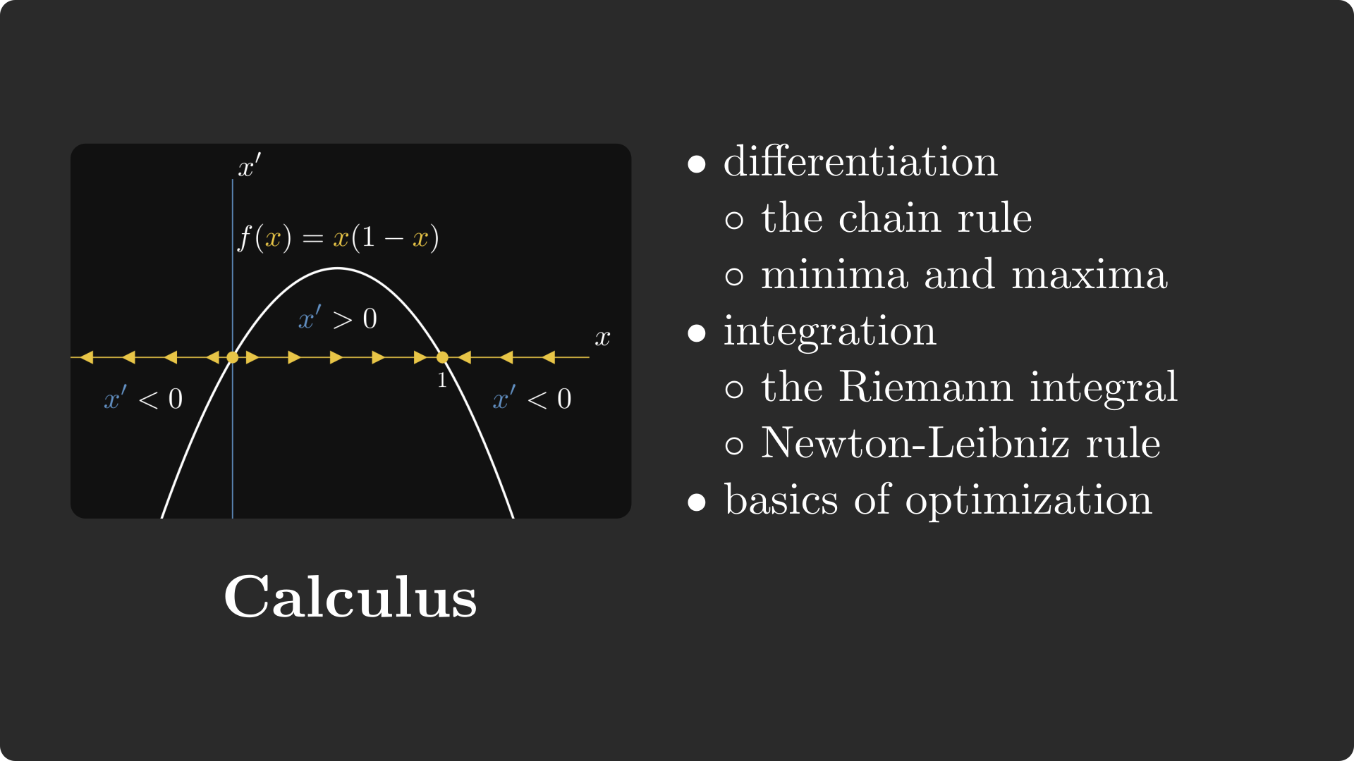
Calculus
Calculus is the study of differentiation and integration of functions. Essentially, a neural network is a differentiable function, so calculus will be a fundamental tool to train neural networks, as we will see.
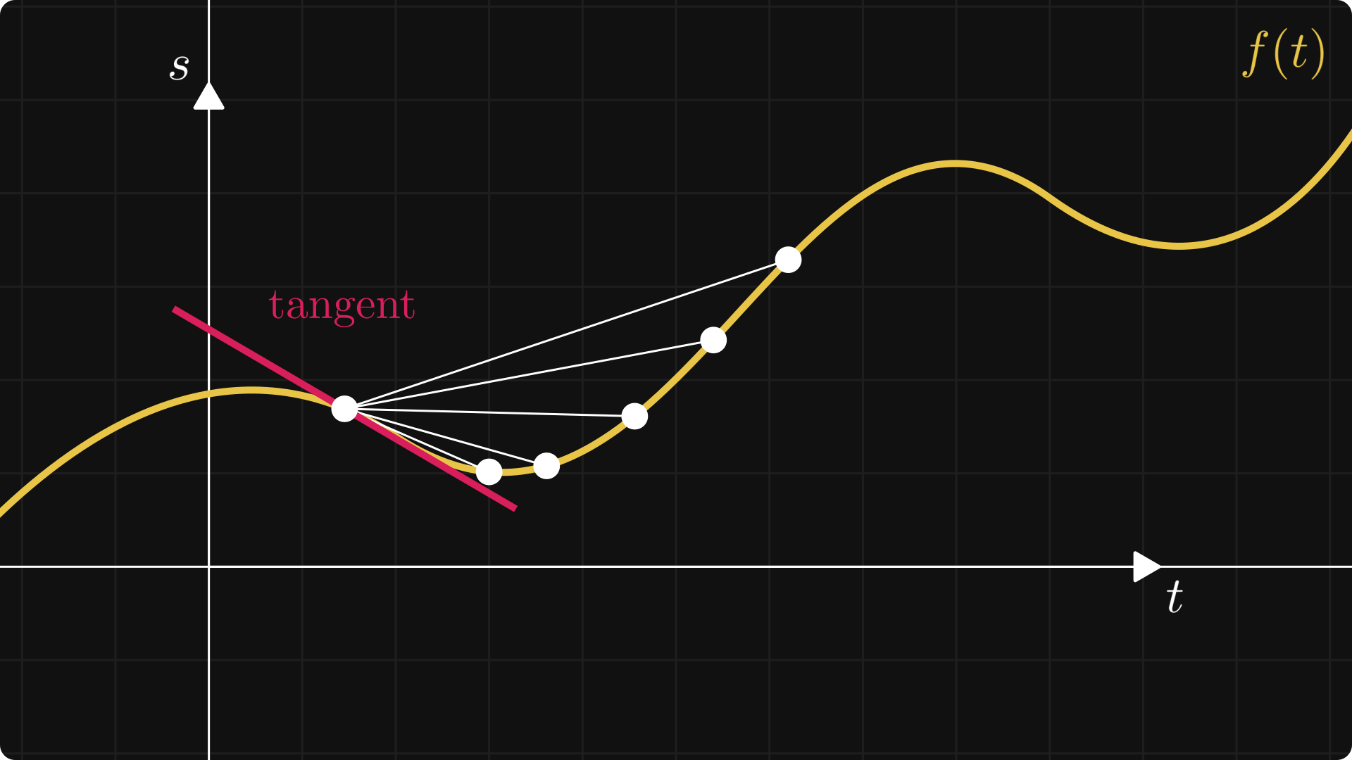
To familiarize yourself with the concepts, you should make things simple and study functions of a single variable for the first time. By definition, the derivative of a function is defined by the limit
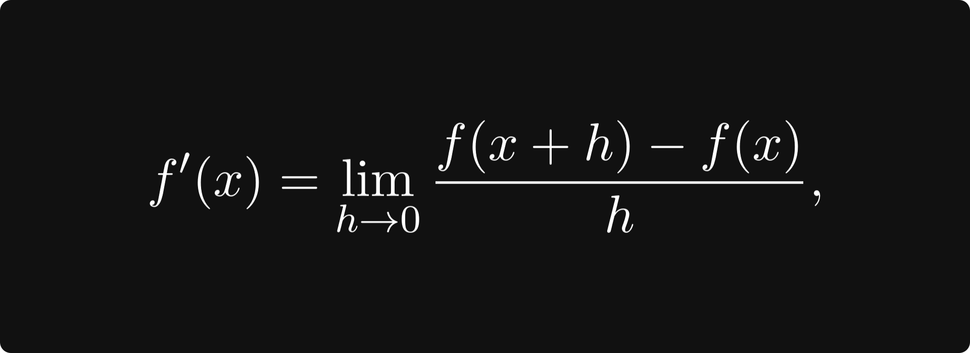
where the ratio for a given h is the slope of the line between the points (x, f(x)) and (x+h, f(x+h)).
In the limit, this is essentially the slope of the tangent line at the point x. The figure below illustrates the concept.
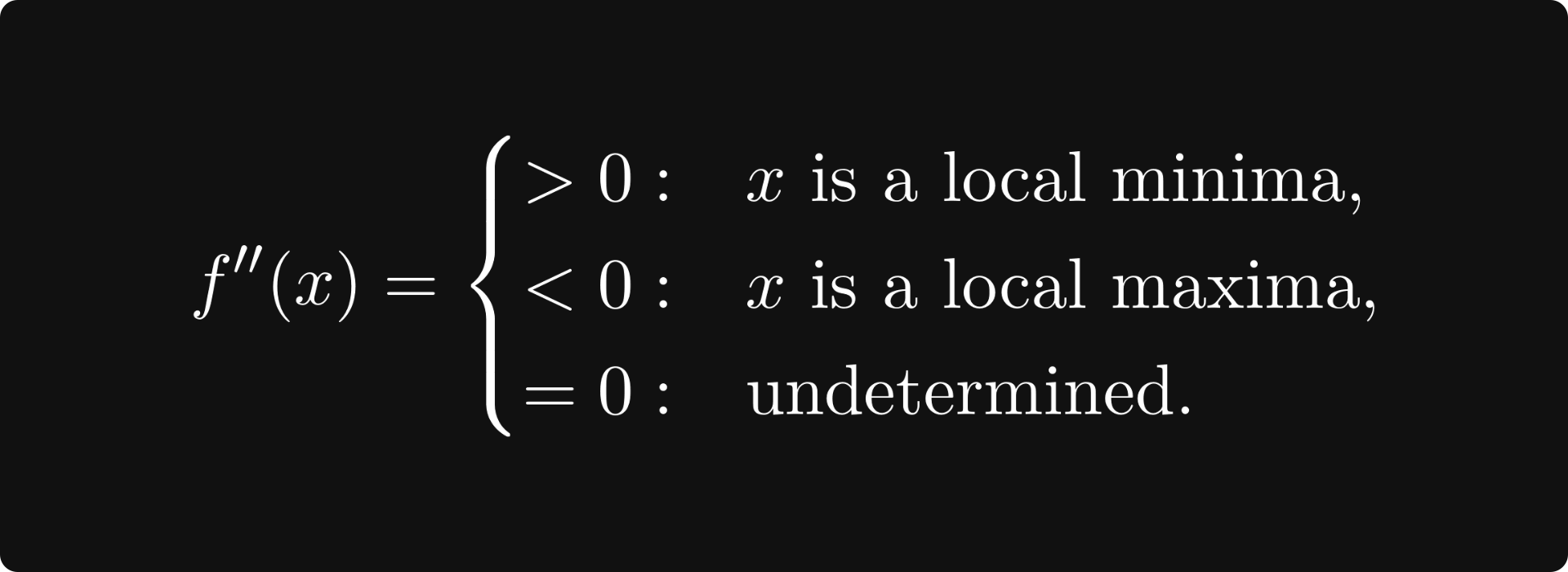
Differentiation can be used to optimize functions: the derivative is zero at local maxima or minima. (However, this is not true in the other direction; see f(x) = x³ at 0.)
Points where the derivative is zero are called critical points. Whether a critical point is a minimum or a maximum can be decided by looking at the second derivative:
There are several essential rules regarding differentiation, but probably the most important is the so-called chain rule:
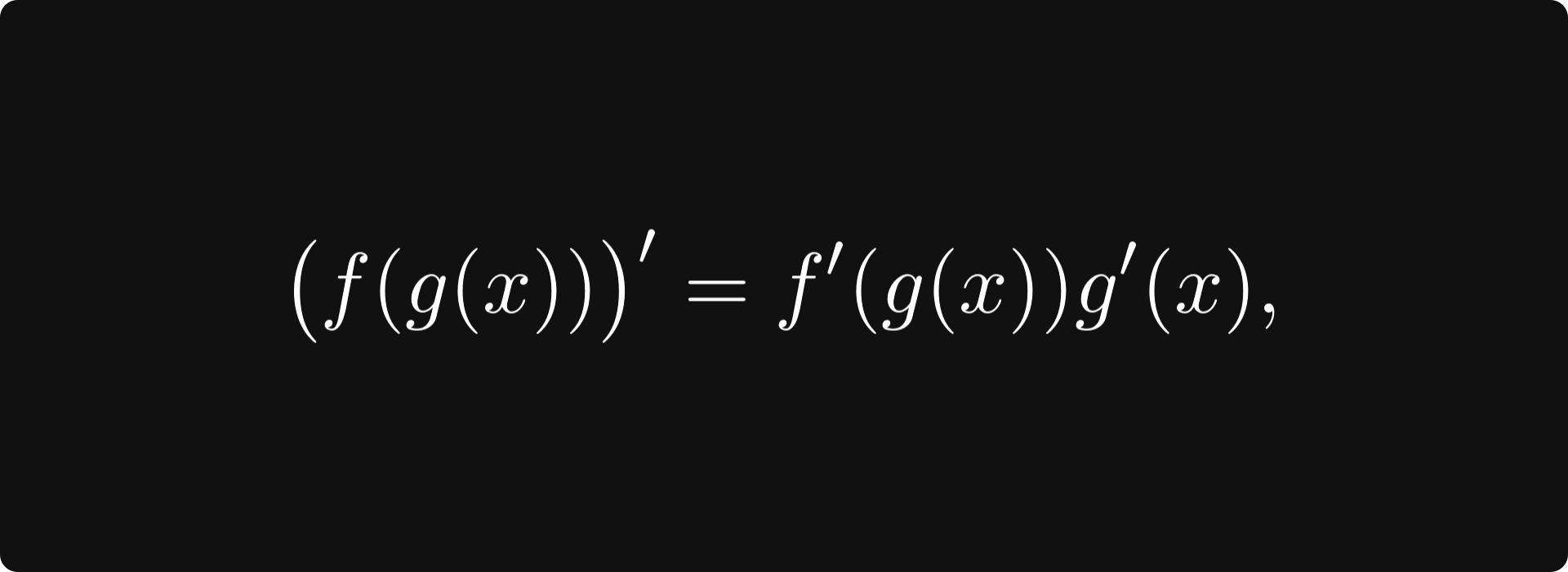
which tells us how to calculate the derivative of composed functions.
Integration is often called the inverse of differentiation. This is true because if f is the derivative of F, that is, F′(x) = f(x), then
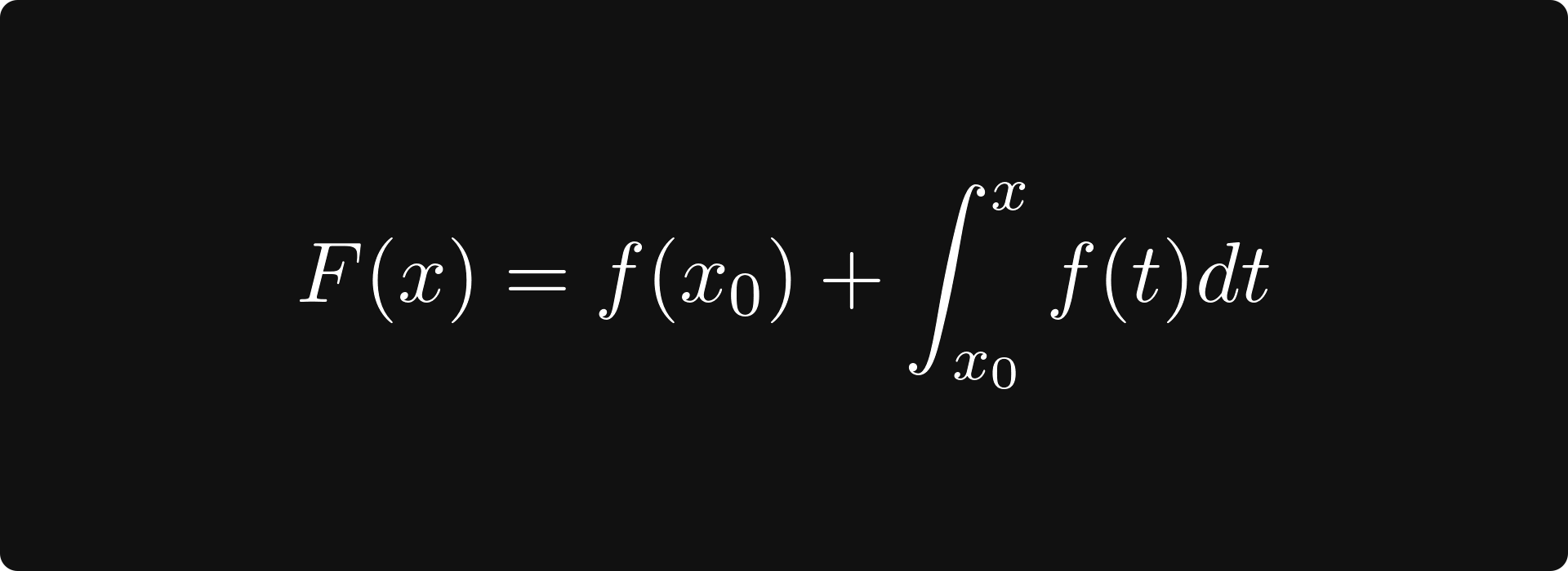
holds. (If f is an integrable function.)
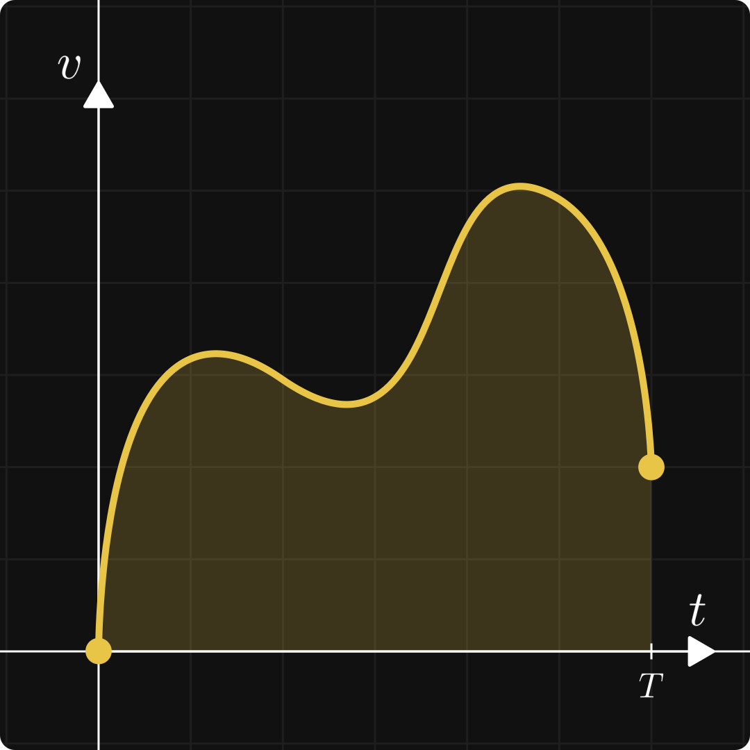
The integral of a function can also be thought of as the signed area under the curve:
Integration itself plays a role in understanding the concept of expected value. For instance, quantities like entropy and Kullback-Leibler divergence are defined in terms of integrals.
Further study
I would recommend the Single Variable Calculus course from MIT. (In general, online courses from MIT are always excellent learning resources.) If you are more of a book person, there are many textbooks available. The Calculus book by Gilbert Strang, which accompanies the previously mentioned course, is again a great resource, available completely free of charge.
Here are some of my articles on the topic:
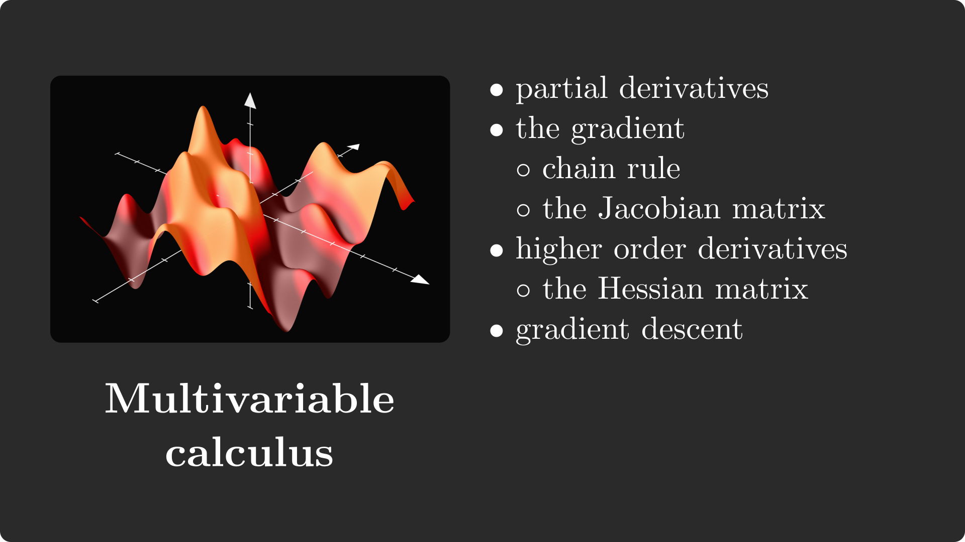
Multivariable calculus
This is the part where linear algebra and calculus come together, laying the foundations for the primary tool to train neural networks: gradient descent. Mathematically speaking, a neural network is simply a function of multiple variables. (Although the number of variables can be in the millions.)
Similar to univariate calculus, the two main topics here are differentiation and integration. Let’s suppose that we have a function f: ℝⁿ → ℝ, mapping vectors to real numbers.
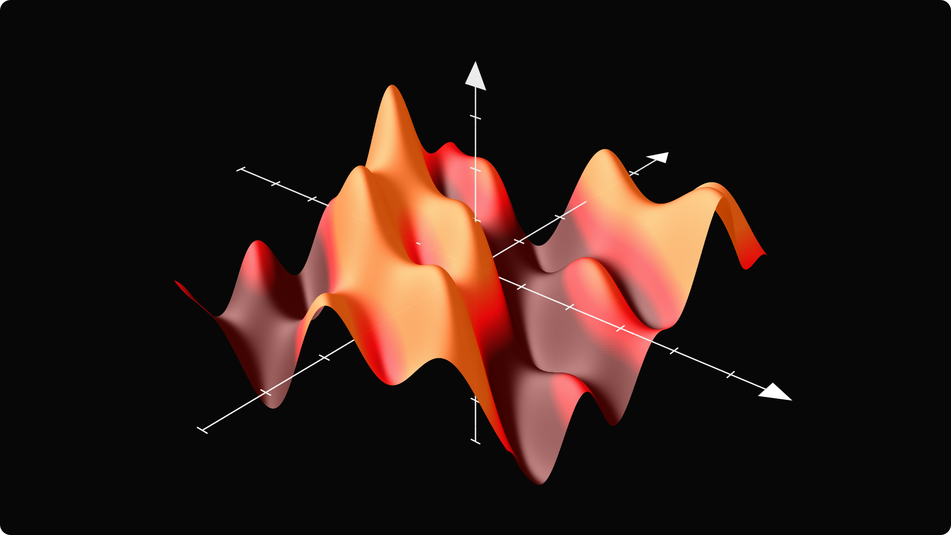
In two dimensions (that is, for n = 2), you can imagine its plot as a surface. (Since humans don’t see higher than three dimensions, it is hard to visualize functions with more than two real variables.)
Differentiation in multiple variables
In a single variable, the derivative was the slope of the tangent line. How would you define tangents here? A point on the surface has several tangents, not just one. However, there are two special tangents: one is parallel to the x-z plane, while the other is parallel to the y-z plane. Their slope is determined by the partial derivatives, defined by
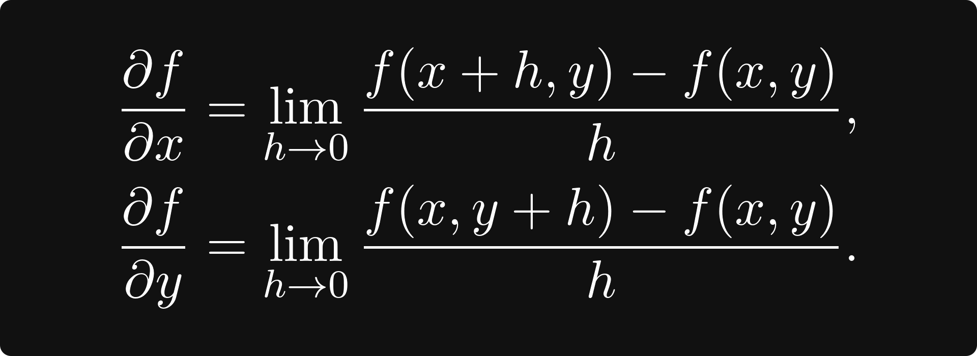
That is, you take the derivative of the functions obtained by fixing all but one variable. (The formal definition is identical for ≥ 3 variables, just more complicated notation.)
Tangents in these special directions span the tangent plane.

The gradient
There is another special direction: the gradient, which is the vector defined by
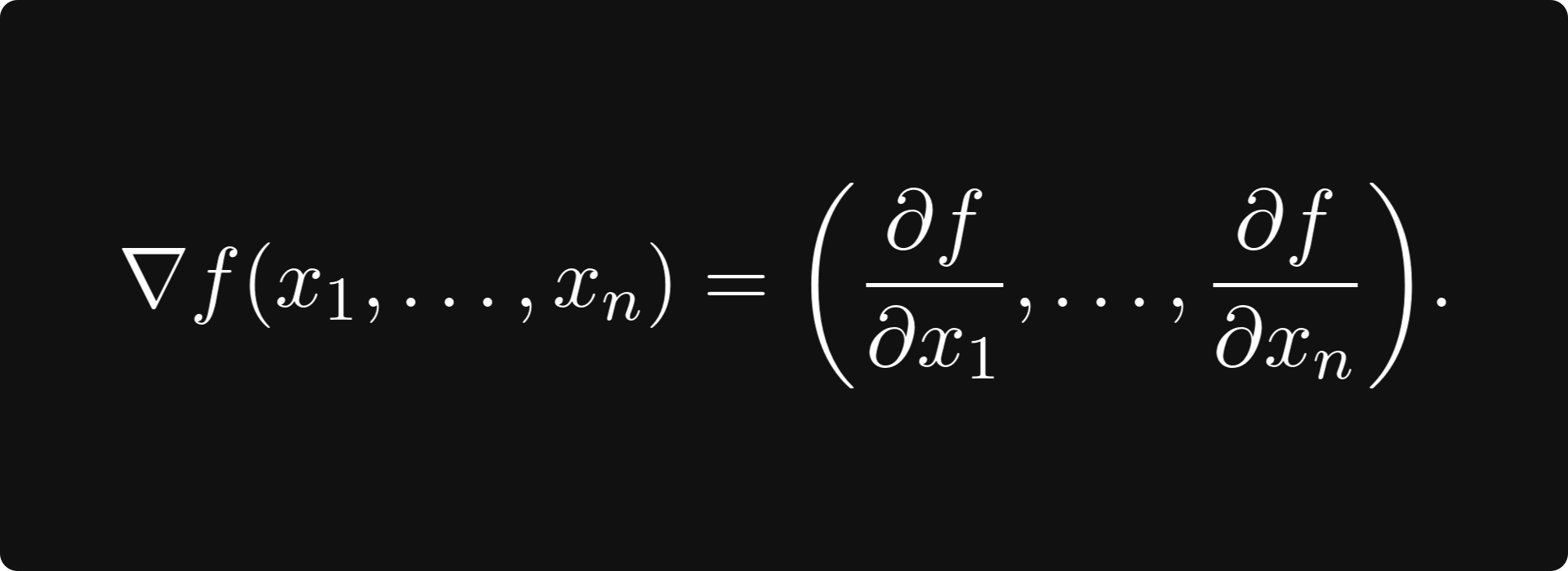
The gradient always points to the direction of the largest increase! So, if you would take a tiny step in this direction, your elevation would be the maximal among all the other directions you could have chosen. This is the basic idea of gradient descent, an algorithm used to maximize functions. Its steps are the following.
Calculate the gradient at the point x₀, where you currently are.
Take a small step in the direction opposite to the gradient to arrive at the point x₁. (The step size is called the learning rate.)
Go back to Step 1 and repeat the process until convergence.
Of course, there are several flaws in this basic algorithm, which has been improved several times over the years. Modern gradient descent-based optimizers employ various techniques, such as adaptive step size, momentum, and other methods, which we will not detail here.
Calculating the gradient in practice is difficult. Functions are often described by the composition of other functions, for instance, the familiar linear layer
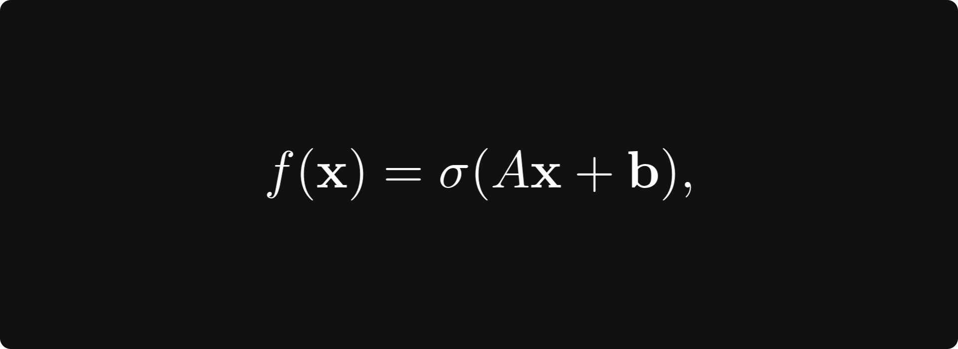
where A is a matrix, b and x are vectors, and σ is the sigmoid function. (Of course, there can be other activations, but we shall stick to this for simplicity.) How would you calculate this gradient? At this point, it is not even clear how to define the gradient for vector-vector functions such as this, so let’s discuss!
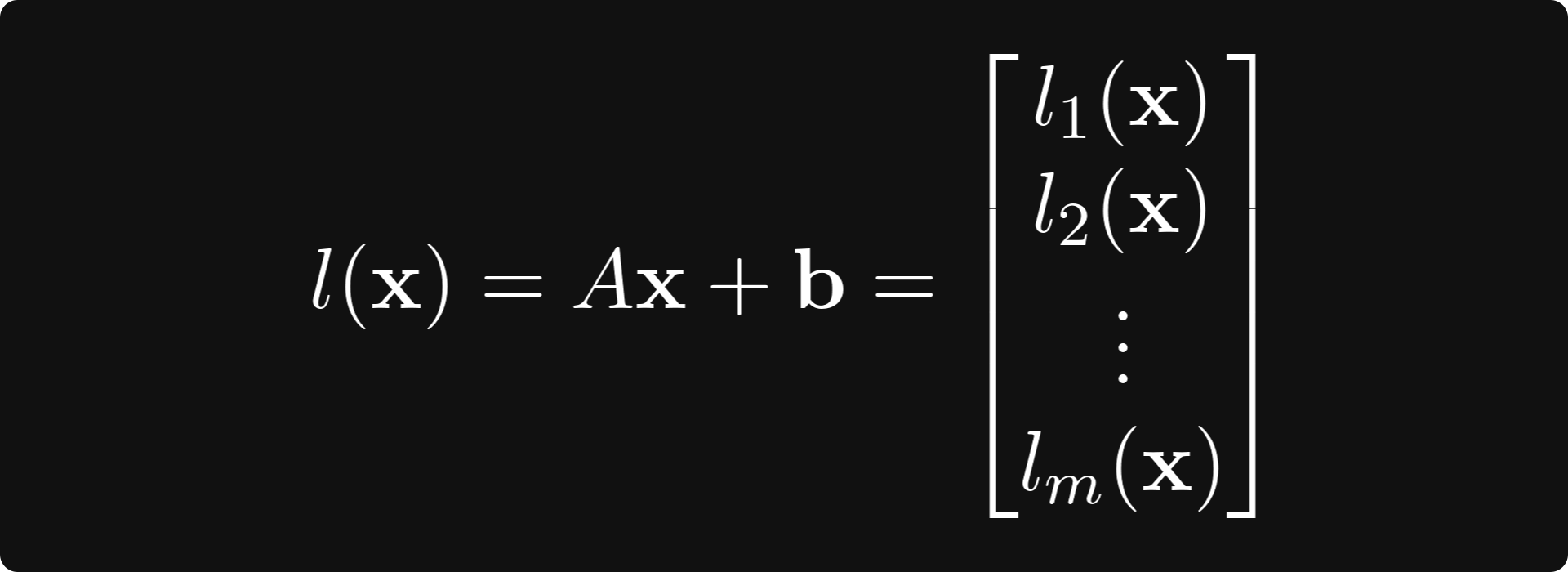
The function g(x): ℝⁿ → ℝᵐ can always be written in terms of vector-scalar functions like
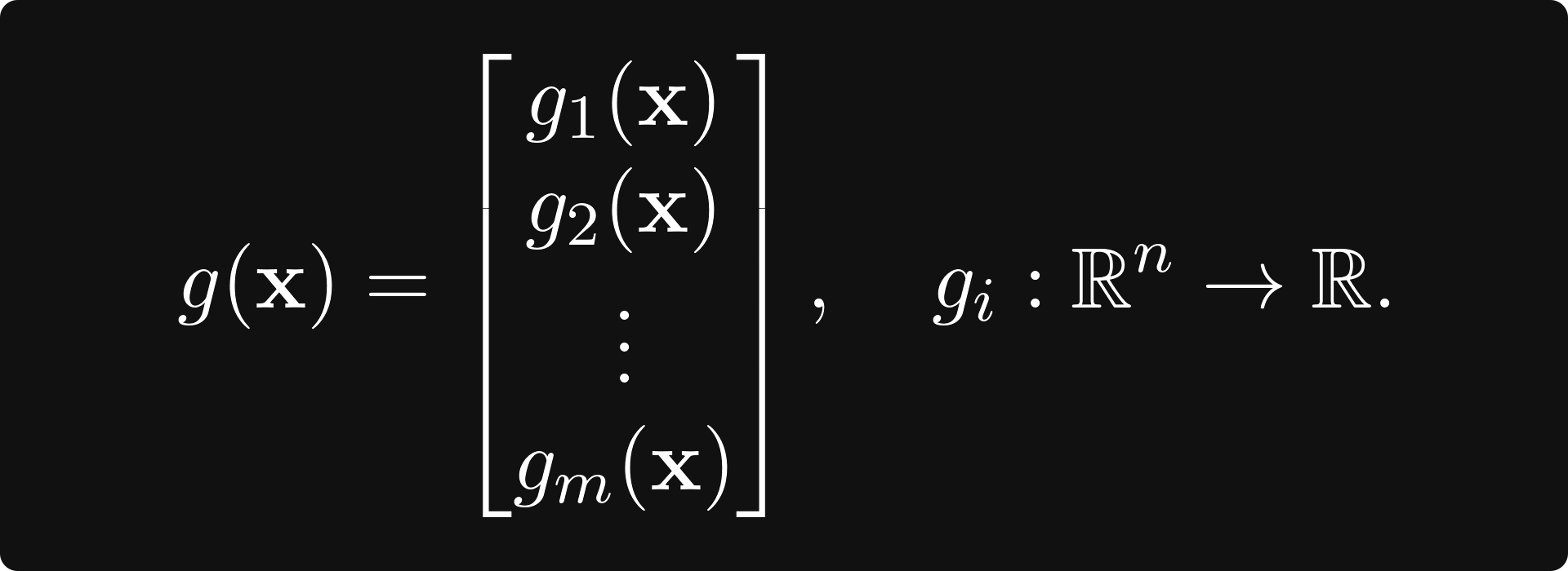
The gradient of g is defined by the matrix whose k-th row is the k-th component’s gradient. That is,
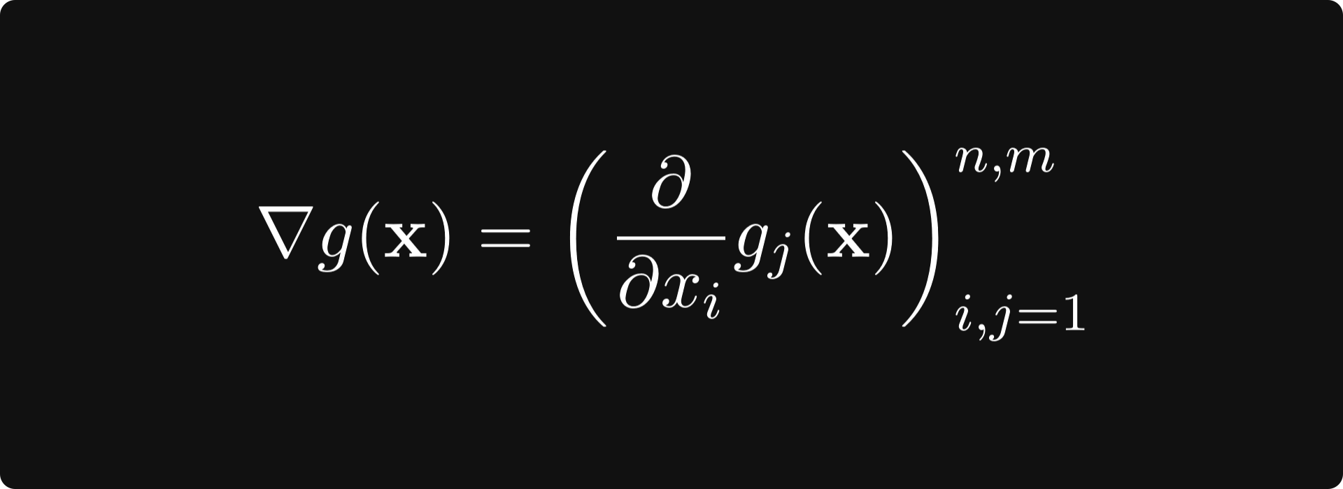
This matrix is called the total derivative of g.
In our example f(x) = σ(Ax + b), things become a bit more complicated because it is the composition of two functions:
l(x) = Ax + b,
and σ(x),
defined by applying the univariate sigmoid componentwise. The function l can be decomposed further to m functions mapping from the n-dimensional vector space to the space of real numbers:
where
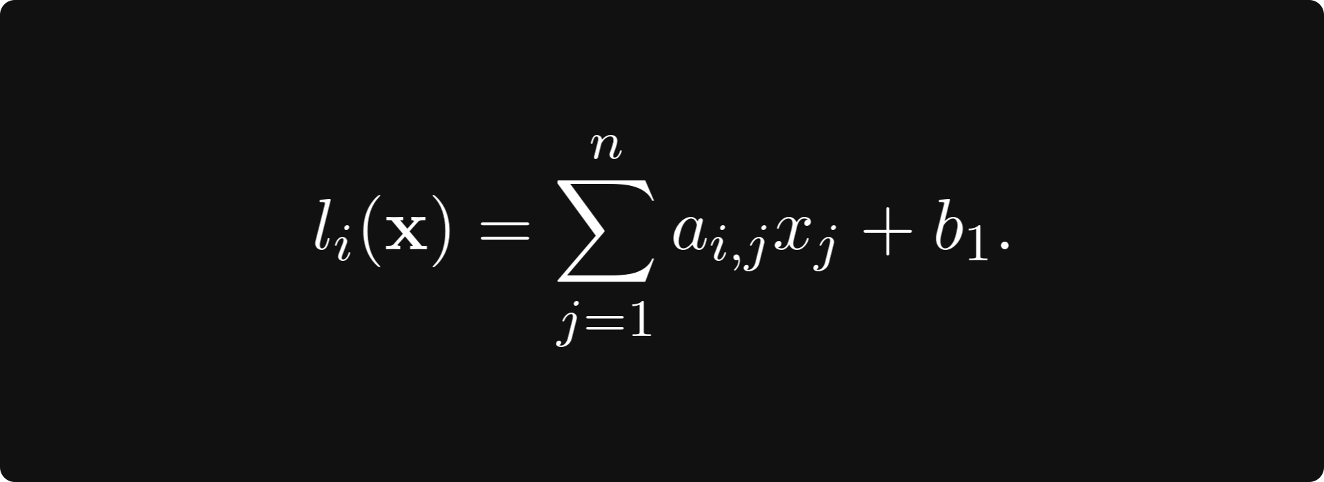
If you calculate the total derivative, you’ll see that
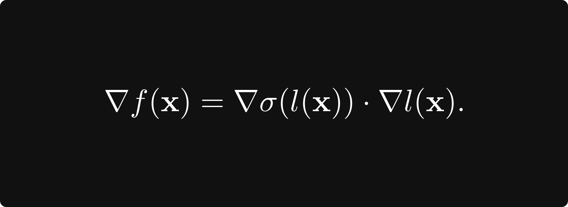
This is the chain rule for multivariate functions in its full generality. Without it, there would be no easy way to calculate the gradient of a neural network, which is ultimately a composition of many functions.
Higher-order derivatives
Similarly to the univariate case, the gradient and derivatives play a role in determining whether a given point in space is a local minimum or maximum. (Or neither.) To provide a concrete example, training a neural network is equivalent to minimizing the loss function on the parameters’ training data. It is all about finding the optimal parameter configuration w for which the minimum is attained:
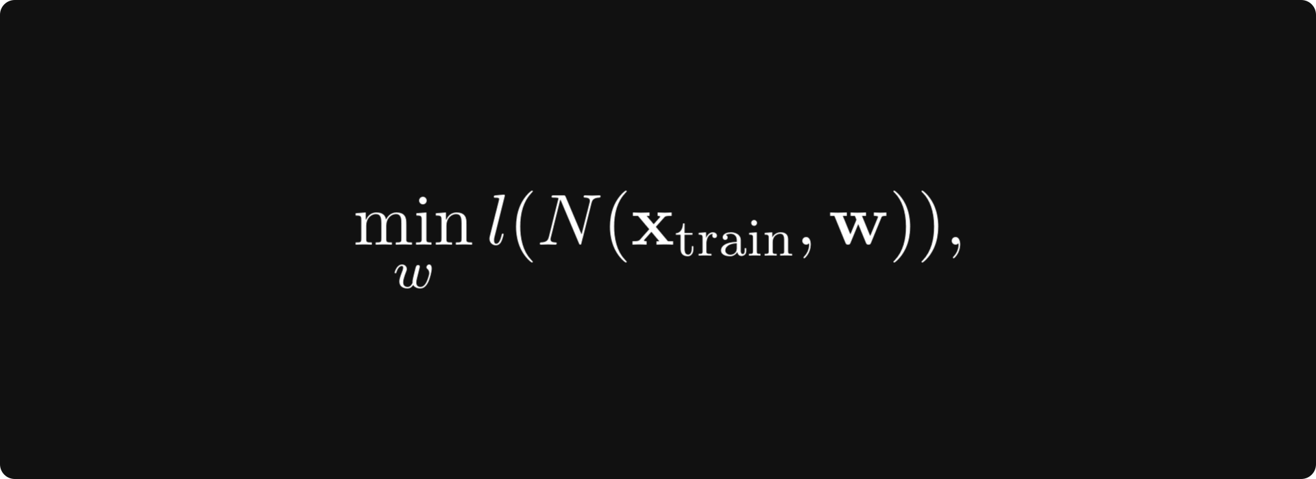
where N: ℝⁿ → ℝᵐ and l: ℝᵐ → ℝ are the neural network and the loss function, respectively.
For a general differentiable vector-scalar function of n variables, there are n² second derivatives, forming the Hessian matrix
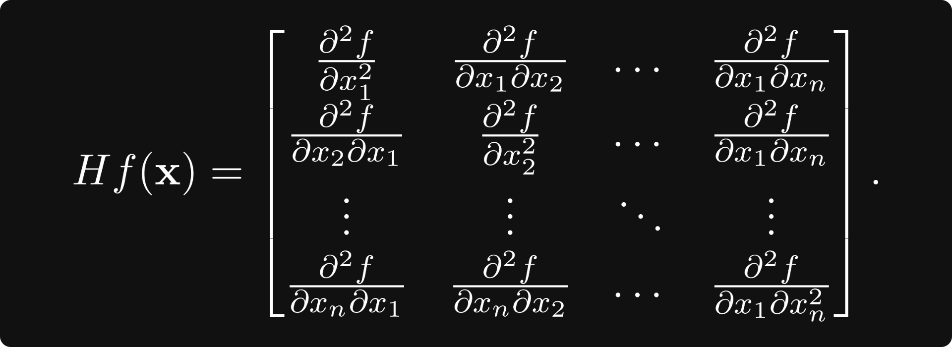
In multiple variables, the determinant of the Hessian takes the role of the second derivative. Similarly, it can be used to determine whether a critical point (i.e., where all the derivatives are zero) is a minimum, maximum, or just a saddle point.
Further study
There are lots of fantastic online courses on multivariable calculus. I have two specific recommendations:
Now we are ready to take on the final subject: probability theory!
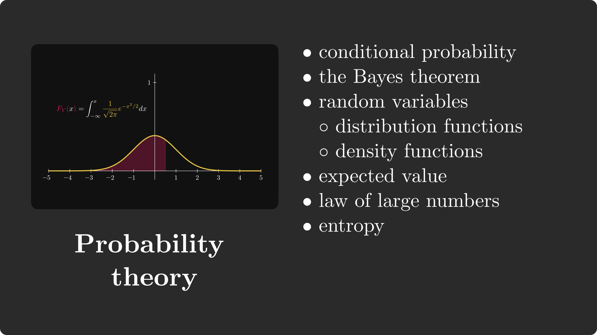
Probability theory
Probability theory is the mathematically rigorous study of chance, fundamental to all fields of science.
Setting exact definitions aside for now, let’s ponder a bit about what probability represents. Let’s say I toss a coin, with a 50% chance (or 0.5 probability) of it being heads. After repeating the experiment 10 times, how many heads did I get?
If you have answered 5, you are wrong. Heads being 0.5 probability doesn’t guarantee that every second throw is heads. Instead, what it means that if you repeat the experiment n times where n is a really large number, the number of heads will be very close to n/2.
Besides the basics, there are some advanced things you need to understand, first and foremost, expected value and entropy. But let’s not get ahead of ourselves! First, we have to understand what probability is!
The concept of probability
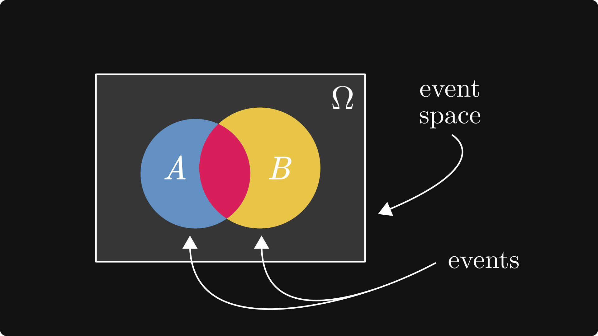
First of all, probability is a function that renders a numeric value between 0 and 1 to events. Events are represented by sets, which are subsets in the event space, denoted by Ω.
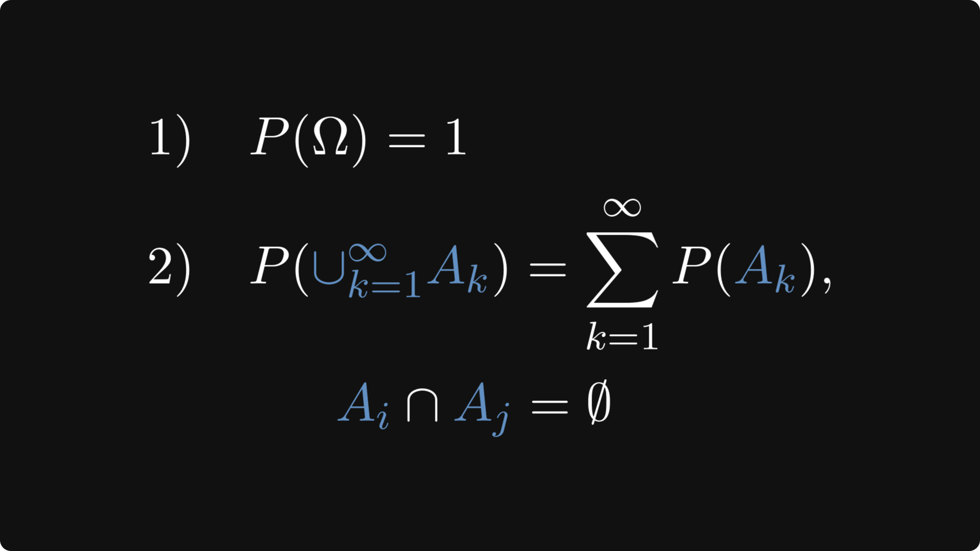
There are two defining properties of probability:
the probability of the entire event space is 1,
and the probabilities of disjoint events can be summed up.
In terms of mathematical formulas:
Set operations can also be translated to the language of events: A ∪ B means that either A or B occurs, while A ∩ B means that both occur.
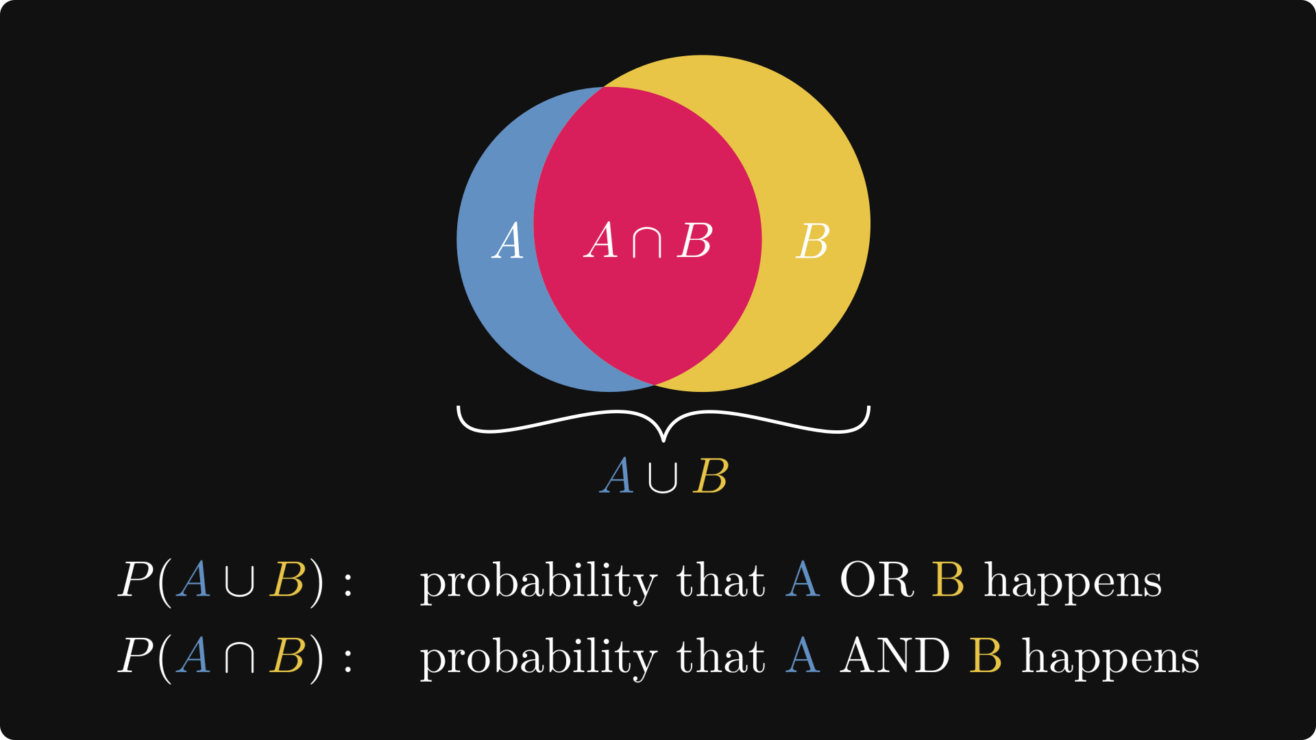
One of the most important concepts in probability theory is conditional probability, which studies probabilities in the context of observations. By definition, it is given by the ratio of the probability of both events occurring and the probability of the observed event.
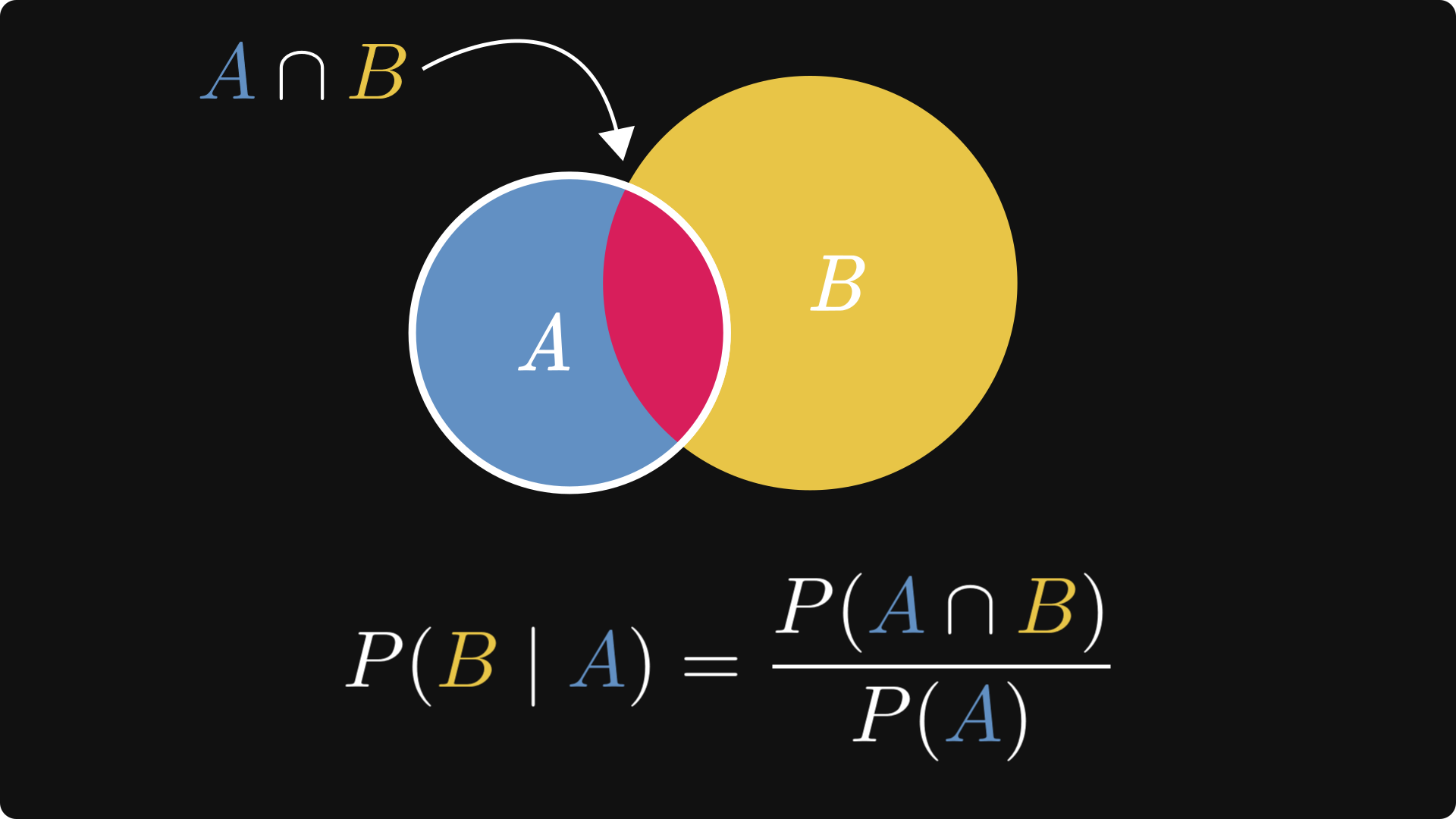
One simple example: what is the probability of a given email being spam, if it contains the word “deal”? Observing keywords like the mentioned “deal” increases the probability of the email being spam.
In certain practical scenarios, we only know P(A | B), but we want to estimate P(B | A). This is what Bayes’ theorem is for, expressing one in terms of the other.
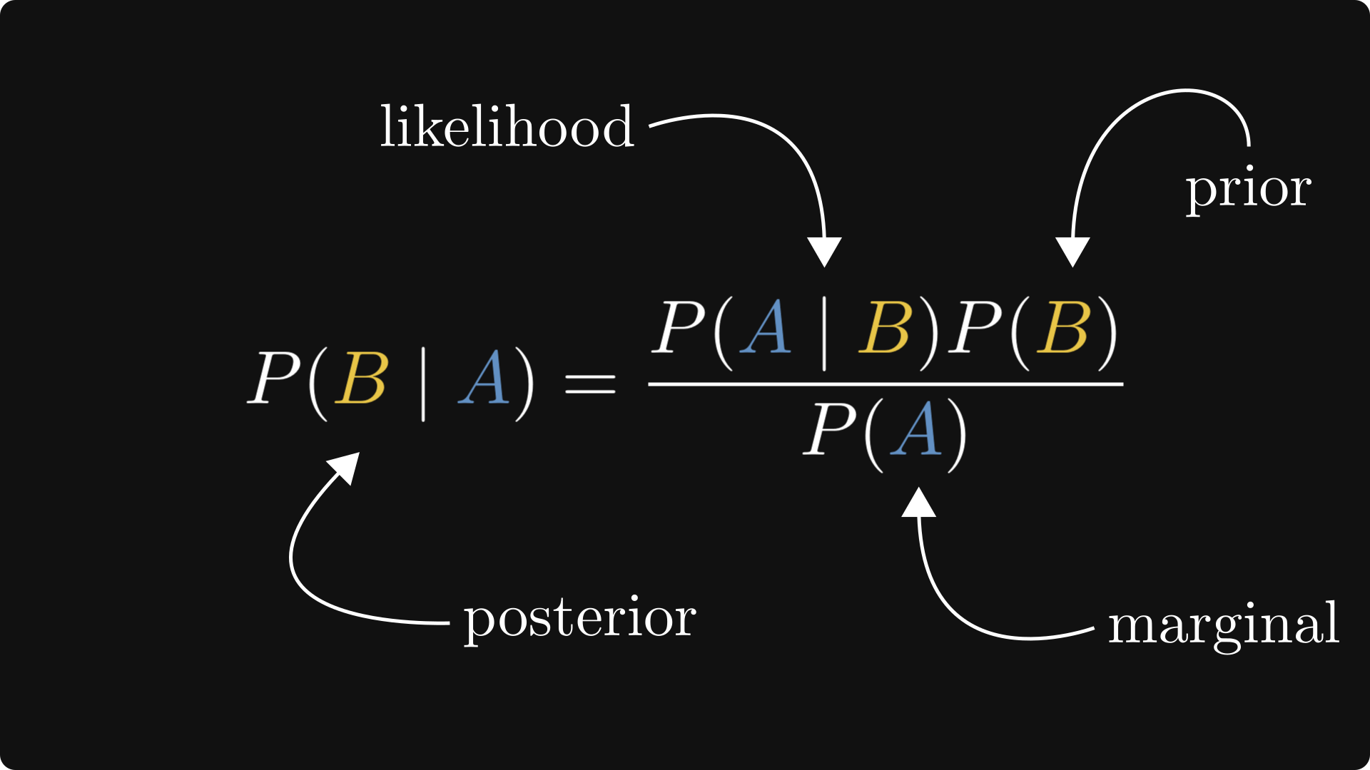
In English, Bayes’ theorem shows us how to update our priors in terms of the likelihood.
Expected value
Suppose that you play a game with your friend. You toss a classical six-sided dice, and if the outcome is 1 or 2, you win 300 bucks. Otherwise, you lose 200. What are your average earnings per round if you play this game long enough? Should you even be playing this game?
Well, you win 100 bucks with probability 1/3, and you lose 200 with probability 2/3. That is, if X is the random variable encoding the result of the dice throw, then
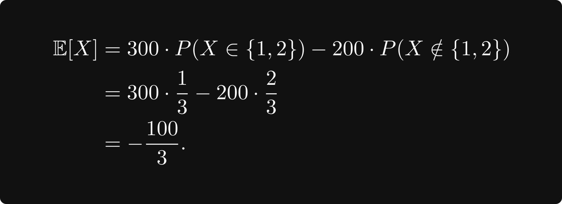
This is the expected value, that is, the average amount of money you will receive per round in the long run. Since this is negative, you will lose money, so you should never play this game.
Generally speaking, the expected value is defined by
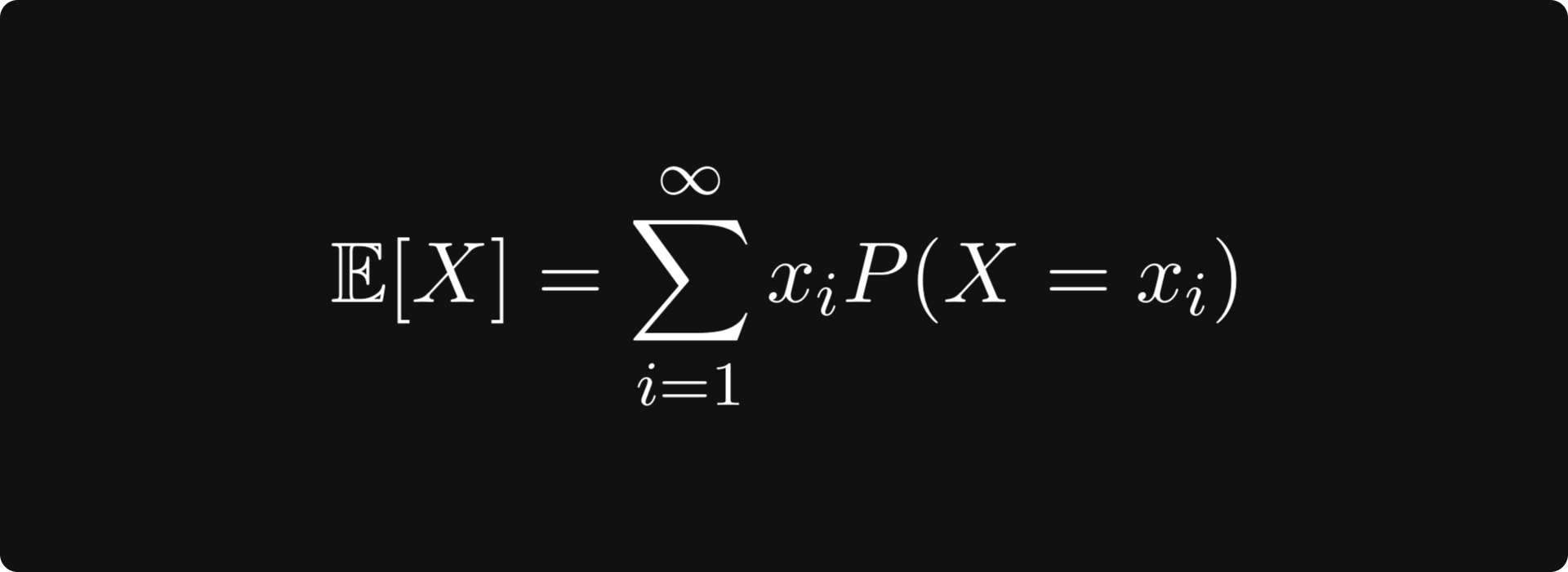
for discrete random variables and
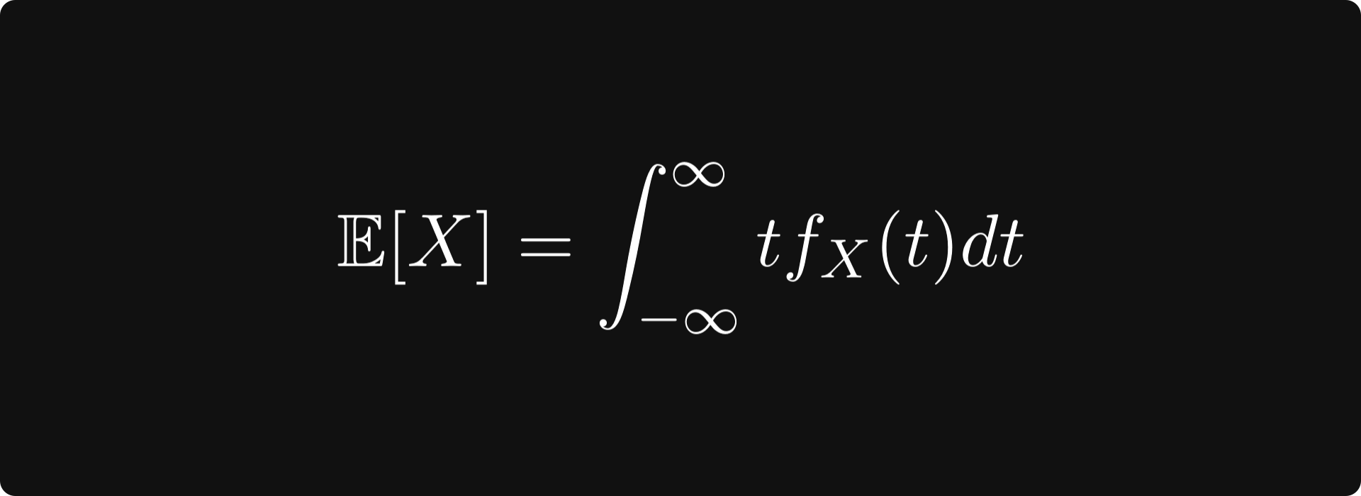
for real-valued continuous random variables.
In machine learning, loss functions for training neural networks are expected values in one way or another.
Law of large numbers
People often falsely attribute certain phenomena to the law of large numbers. For instance, gamblers who are on a losing streak believe that they should soon win because of the law of large numbers. This is totally wrong. Let’s see what this is really!
Suppose that X, X₁, X₂, ... are random variables representing the independent repetitions of the same experiment. (Say, rolling a dice or tossing a coin.)
The (strong) law of large numbers states that
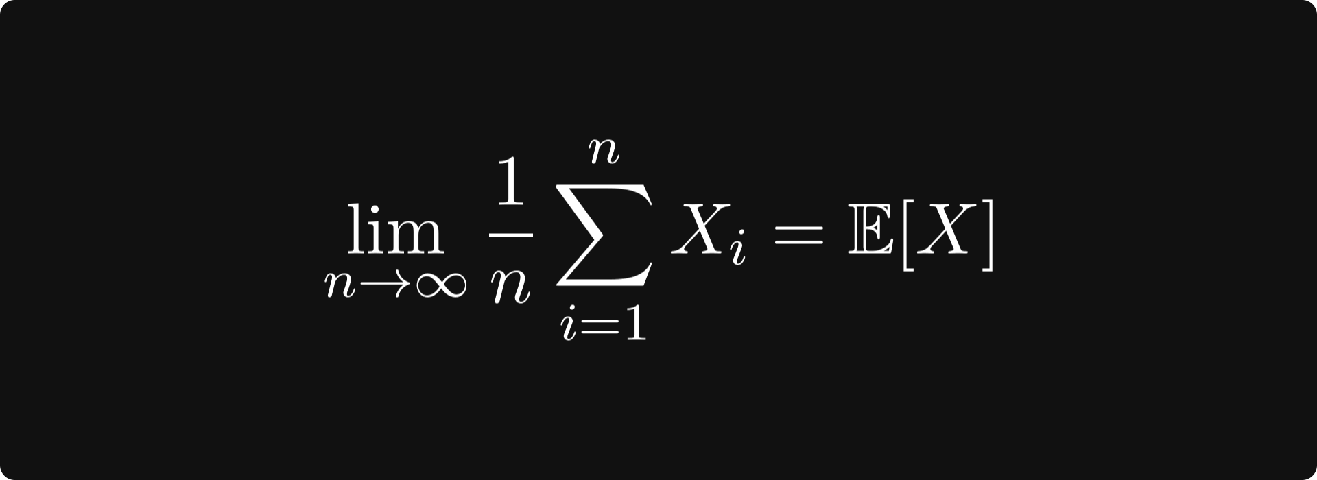
holds with probability one; that is, the average of the outcomes in the long run equals the expected value.
An interpretation is that if a random event is repeated enough times, individual results might not matter. So, if you are playing in a casino with a game that has negative expected value (as they all do), it doesn’t matter that you win occasionally. The law of large numbers implies that you will lose money.
To get a little bit ahead, LLN is going to be essential for stochastic gradient descent.
Information theory
Let’s play a game. I have thought of a number between 1 and 1024, and you have to guess it. You can ask questions, but your goal is to use as few questions as possible. How much do you need?
If you play it smart, you will perform a binary search with your questions. First, you may ask: is the number between 1 and 512? With this, you have cut the search space in half. Using this strategy, you can figure out the answer in log₂(1024) = 10 questions.
But what if I didn’t use the uniform distribution when picking the number? For instance, I could have used a Poisson distribution.
Here, you would probably need fewer questions because you know that the distribution tends to concentrate around specific points. (Which depends on the parameter.)
In the extreme case, when the distribution is concentrated on a single number, you need zero questions to guess it correctly. Generally, the number of questions depends on the information carried by the distribution. The uniform distribution contains the least amount of information, while singular ones are pure information.
Entropy is a measure that quantifies this. It is defined by

for discrete random variables and
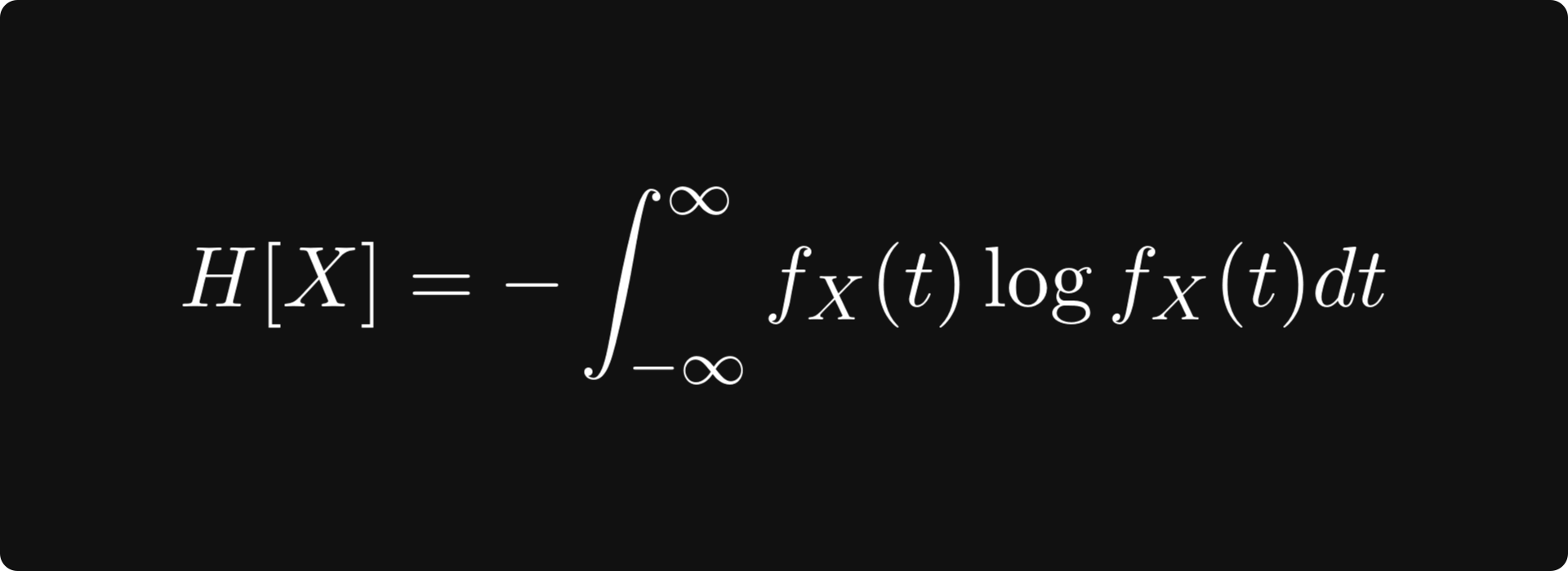
for continuous, real-valued ones. (The base of the logarithm is usually 2, e, or 10, but it doesn’t really matter.)
If you have ever worked with classification models before, you probably encountered the cross-entropy loss, defined by
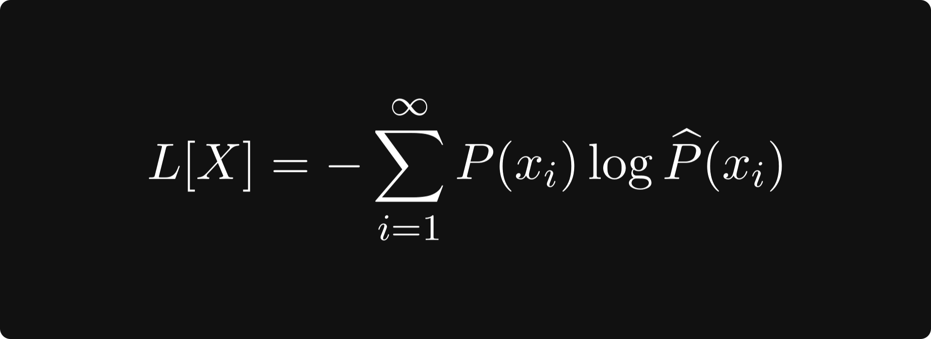
where P is the ground truth (a distribution concentrated to a single class), while the hatted version represents the class predictions. The cross-entropy loss measures how much “information” the predictions have compared to the ground truth. When the predictions match, the cross-entropy loss is zero.
Another frequently used quantity is the Kullback-Leibler divergence, defined by
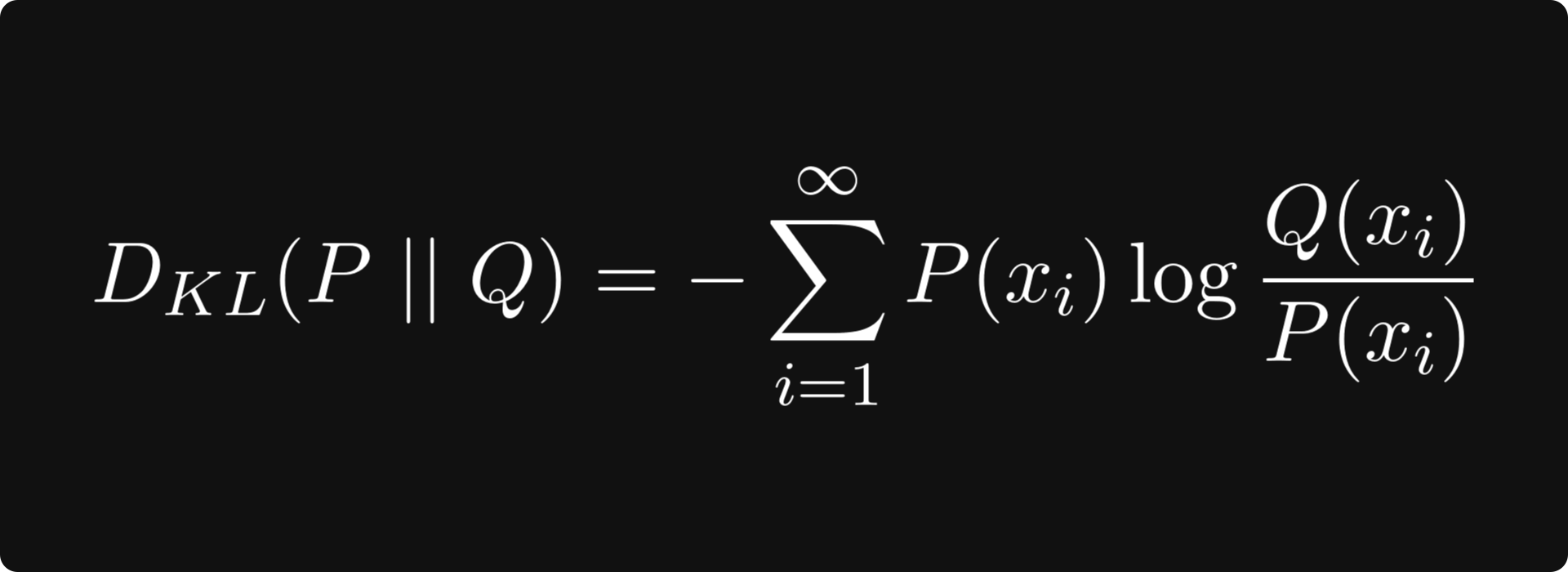
where P and Q are two probability distributions. This is essentially cross-entropy minus the entropy, which can be thought of as quantifying the difference between the two distributions. This is useful, for instance, when training generative adversarial networks. Minimizing the Kullback-Leibler divergence guarantees that the two distributions are similar.
Further study
Here, I would again recommend an online course from MIT, which covers all the fundamentals and some advanced concepts. Check out Introduction to Probability by John Tsitsiklis!
Some of my articles about probability:
P.S. If you want a single resource with a full breakdown of this entire roadmap, consider buying my book, The Mathematics of Machine Learning.
Outstanding resource. Thanks!
Small typo in figure. c^2 = a^2 + b^2, not the square root of ...