The Maximum Likelihood Estimation
(is the foundation of machine learning)
This post is the next chapter of my upcoming Mathematics of Machine Learning book, available in early access.
New chapters are available for the premium subscribers of The Palindrome as well, but there are 40+ chapters (~500 pages) available exclusively for members of the early access.
I am an evangelist for simple ideas. Stop me any time you want, but whichever field I was in, I've always been able to find a small set of mind-numbingly simple ideas making the entire shebang work. (Not that you could interrupt me, as this is a book. Joke's on you!)
Let me give you a concrete example that's on my mind. What do you think enabled the rise of deep learning, including neural networks with billions of parameters? Three ideas as simple as ABC:
that you can optimize the loss function by going against its gradient (no matter the number of parameters),
that you can efficiently compute the gradient with a clever application of the chain rule and matrix multiplication,
and that we can perform matrix operations blazing fast on a GPU.
Sure, there's a great tower of work built upon these ideas, but these three lie at the very foundation of machine learning today. Ultimately, these enable you to converse with large language models. To have your car cruise around the town while you're reading newspapers. To predict the exact shape of massive amino-acid chains called proteins, responsible for building up every living thing. (Including you.)
Gradient descent, backpropagation, and high-performance linear algebra are on the practical side of the metaphorical machine learning coin. If we conjure up a parametric model, we can throw some extremely powerful tools to it.
But how on earth do we get our models from?
As I've said, there is a small set of key ideas that go a long way. We are about to meet our first one: the maximum likelihood estimation.
Probabilistic modeling 101
As a self-proclaimed evangelist of simple ideas, I'll start with a simple example to illustrate a simple idea.
Pick up a coin and toss it a few times, recording each outcome. The question is, once more, simple: what's the probability of heads? We can't just immediately assume p = 1/2, that is, a fair coin. For instance, one side of our coin can be coated with lead, resulting in a bias. To find out, let's perform some statistics. (Rolling up my sleeves, throwing down my gloves.)
Mathematically speaking, we can model coin tosses with the Bernoulli distribution: P(X = 1) = p, and P(X = 0) = 1 - p,
where
X is the random variable representing the outcome of a single toss,
X = 1 for heads and X = 0 for tails,
and p [0, 1] is the probability of heads.
That's just the model. We're here to estimate the parameter p, and this is what we have statistics for.
Tossing up the coin n times yields the zero-one sequence x₁, x₂, …, xₙ, where each xᵢ is a realization of a Bernoulli-distributed random variable Xᵢ ~ Bernoulli(p), independent of each other.
One natural idea is to compute the sample mean to estimate p, which is coincidentally the expected value of X. To move beyond empirical estimates, let's leverage that this time, it's personal we have a probabilistic model.
The key question is this: which parameter p is the most likely to produce our sample?
In the language of probability, this question is answered by maximizing the likelihood function
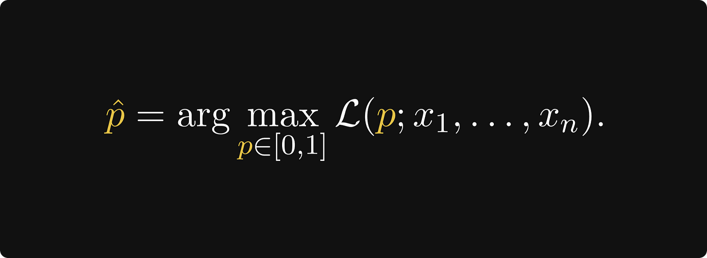
where P(Xᵢ = xᵢ | p) is the probability of xᵢ a fixed value of the parameter p. The larger the L(p; x₁, …, xₙ), the more likely the parameter p is. In other words, our estimate of p is going to be
Let's find it.
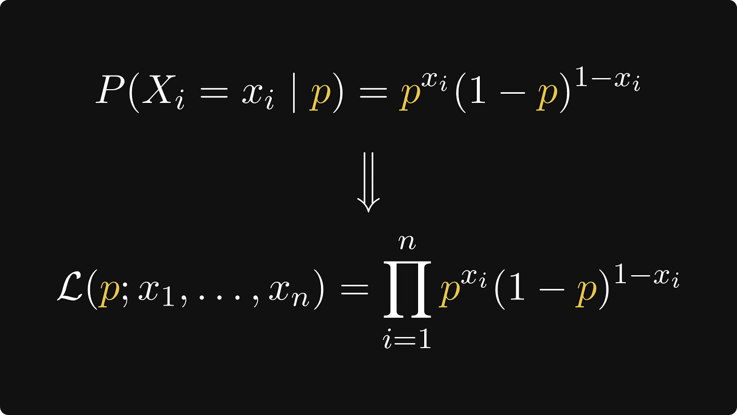
In our concrete case, P(Xᵢ = xᵢ | p) can be written as
Algebra doesn't welcome if-else type functions, so with a clever mathematical trick, we write P(Xᵢ = xᵢ | p) as a product, making the likelihood function to be
(We'll often write L(p) to minimize notational complexity.)
This is still not easy to optimize, as it is composed of the product of exponential functions. So, here's another mathematical trick: take the logarithm to turn the product into a sum. As the logarithm is increasing, it won't change the optima, so we're good to go:
Trust me, this is much better. According to second derivative test, we can find the maxima by
finding the zeros of the derivative to find the critical points, that is, potential local extrema,
then using the second derivative to find the maximum among the critical points.
Let's get to it.
As (log p)' = 1/p and (log (1 - p))' = -1/(1 - p), we have
The derivative has a single zero:
(Pick up a pen and paper and calculate the solution yourself.) I won’t calculate the second derivative here, but trust me, it confirms that this is indeed a maximum, giving us the maximum likelihood estimate.
In this case, the maximum likelihood estimate is identical to the sample mean. Trust me, this is one of the rare exceptions. Think of it as a validation of the sample mean: different thought processes yield the same estimate, so it must be good.
Modeling heights
Let's continue with another example. The coin-tossing example demonstrated the discrete case. It's time to move into the continuous domain!
This time, we are measuring the heights of a high school class, and we want to build a probabilistic model of it. A natural idea is to assume the heights to come from a normal distribution X ~ N(μ, σ²).
Our job is to estimate the expected value μ and the variance σ². Let's go, maximum likelihood!


