The mathematics of optimization for deep learning
A brief guide to minimize a function with millions of variables
Hi there! I started to write about math and machine learning around the end of 2019; since then, I have written hundreds of educational pieces unraveling the details behind the algorithms we use daily.
One surefire way to make a writer cringe: make them read their earlier works. I am no exception. I came a long way from 2019. (Though I still write at a glacial pace.)
Despite all of this, there are several early posts that I am proud of. Posts where I captured the sweet spot between intuition and precision. Lately, I have been working on remastering the best of them.
Here’s the first one, where we go from zero to optimizing functions with millions of variables. Enjoy!
What contributes the most to a neural network's performance?
This is a complex question, as performance depends on several factors. The one usually taking the spotlight is the network architecture. However, this is only one among many essential components. An often overlooked contributor to a performant algorithm is the optimizer used to fit the model.
To illustrate the complexity of optimizing, consider a ResNet18 architecture with exactly 11689512 parameters. Finding an optimal parameter configuration is the same as locating a point in the 11689512-dimensional space. We can brute force this by
dividing the space up with a grid,
selecting 10 points along each dimension,
and checking 10^11689512 possible parameter configurations by calculating the loss function for each to find the one with minimal loss.
To put the number 10^11689512 in perspective, the observable universe has about 10^83 atoms, estimated to be 4.32 × 10^17 seconds (~13.7 billion years) old. If we check as many parameter configurations in each second as the number of atoms starting from the Big Bang, we would have been able to check 4.32 × 10^1411 points until now.
Not even close. The grid size is still approximately 10^8284 times larger than we could check if we would have every atom in the universe check a configuration since the Big Bang.
So, optimization is pretty important. Without optimizers, deep learning would not be possible. They manage this incomprehensible complexity, allowing us to train the neural networks in days instead of billions of years.
In this post, we'll take a deep dive into the mathematics of optimizers and see how they handle this seemingly impossible task.
The basics of optimization
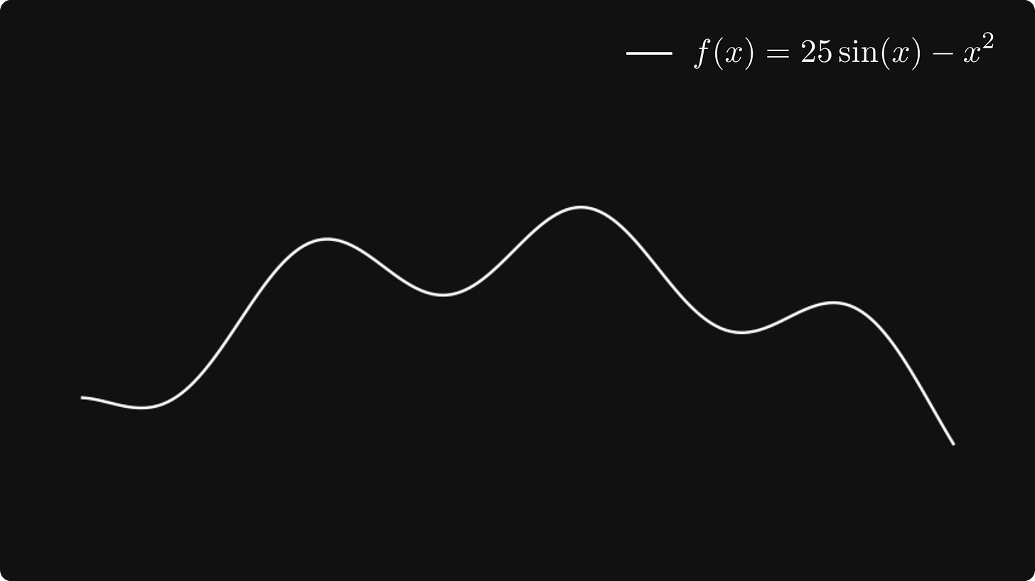
Let's start simple and maximize a function of a single variable. (In a machine learning context, we aim to minimize the loss, but minimizing an f is the same as maximizing -f.) For instance, we define f(x) = 25 · sin(x) - x².
Let’s plot it!
The first idea is to divide the line into a grid, check the value of every point, and select the one where the function is maximized. As we have seen in the introduction, this is not scalable. Thus, we must look for another solution.
Let's imagine that the function is a mountain landscape, and we are climbers trying to reach the peak! Suppose that we are at the location marked by a red dot.
If we want to find the peak, which direction should we go? Towards the increase.
The notion of “increase” is formalized by the concept of the derivative. Mathematically, the derivative is defined by
Although this quantity seems mysterious at first glance, it has a straightforward geometric meaning. Let's look at the function more closely around the point x₀, where we take the derivative.
For any x and y, the line passing through f(x) and f(y) is defined by the equation
In general, for the line defined by at + b, the quantity a is called the slope of the line. The slope can be negative and positive as well.
Lines with a positive slope go upward, while negative ones go downward. Higher values in absolute value mean steeper lines. If we let y get closer and closer to x₀ as it is in the definition of derivative, we see that the line becomes the tangent of the function graph at x₀.
The tangent is given by the function
and we can describe its direction by the vector (1, f ’(x)).
If we imagine ourselves again in the position of a mountain climber starting from
x₀ = -2.0, we should go in the direction where the tangent is rising. If the tangent slope is large, we would also like to take a large step, while if the slope is close to zero, we should take a smaller step to make sure we don't go over the peak. To formalize this mathematically, we should go to the next point defined by
where λ > 0 is the parameter called learning rate, setting how large the step should be in the direction of increase.
Think about this: if the derivative f’(x₀) is positive, x₁ moves ion the positive direction. If f’(x₀) is negative, x₁ moves in the negative direction.
Subsequent steps are defined by
Let’s visualize this process!
As we can see, this simple algorithm successfully found a peak!
(However, this is not the global maximum of the function. To get ahead of ourselves, this is a potential issue for a broad family of optimizing algorithms, but there are solutions for it.)
In this simple case, we have only maximized a function of a single variable. This is useful to illustrate the concept. However, in real-life scenarios, millions of variables can be present. For neural networks, this is definitely the case. The next part will show how this simple algorithm can be generalized for optimizing multidimensional functions!
Optimizing in multiple dimensions
For single-variable functions, we can think about the derivative as the slope of the tangent line. However, for multiple variables, this is different.
Let's build our intuition by studying an example! Define the function
which will be our toy example in this section.
Author’s note. Apologies for the inconsistency of the illustrations, but I failed to adapt the multivariable surface plots in Manim. Despite all my efforts to tune the
z_index, I couldn’t manage to correctly render the surface and the tangent planes in the right order.
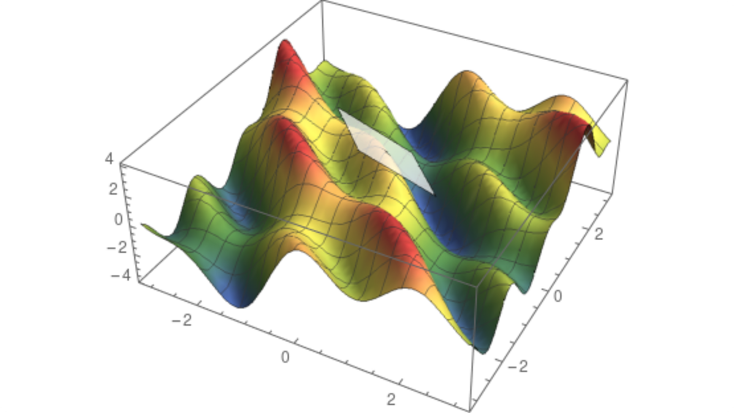
For functions of two variables, the graph is a surface. We immediately see that the concept of the tangent line is not well defined since we have many tangent lines to a given point on the surface. In fact, we have a whole plane of them. This is called the tangent plane.
However, the tangent plane contains two special directions.
Suppose we are looking at the tangent plane at (0, 0). For every multivariable function, fixing all but one variable is a function of a single variable. In our case, we would have the two functions
We can visualize these functions by slicing the surface with a vertical plane perpendicular to one of the axes. Where the plane and the surface meet is the graph of f(x, 0) or f(0, y), depending on which plane you use. This is how it looks.
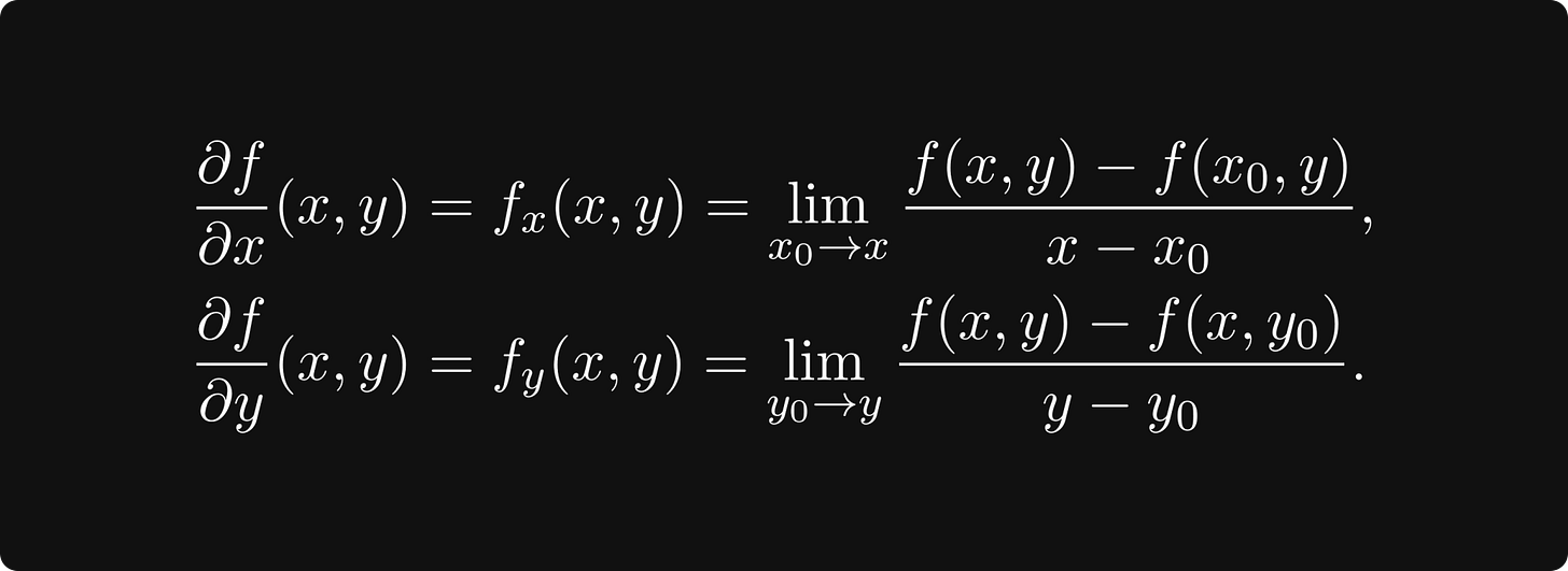
For the single-variable functions f(x, 0) and f(0, y), we define the derivatives as we have done in the previous section. These are called partial derivatives of f(x, y), and they play an essential role in our peak-finding algorithm.
Mathematically, the partial derivatives are defined by
Each partial derivative represents a direction in our tangent plane.
The partial derivatives describe the slopes of the tangent lines for f(x, ·) and f(·, y).
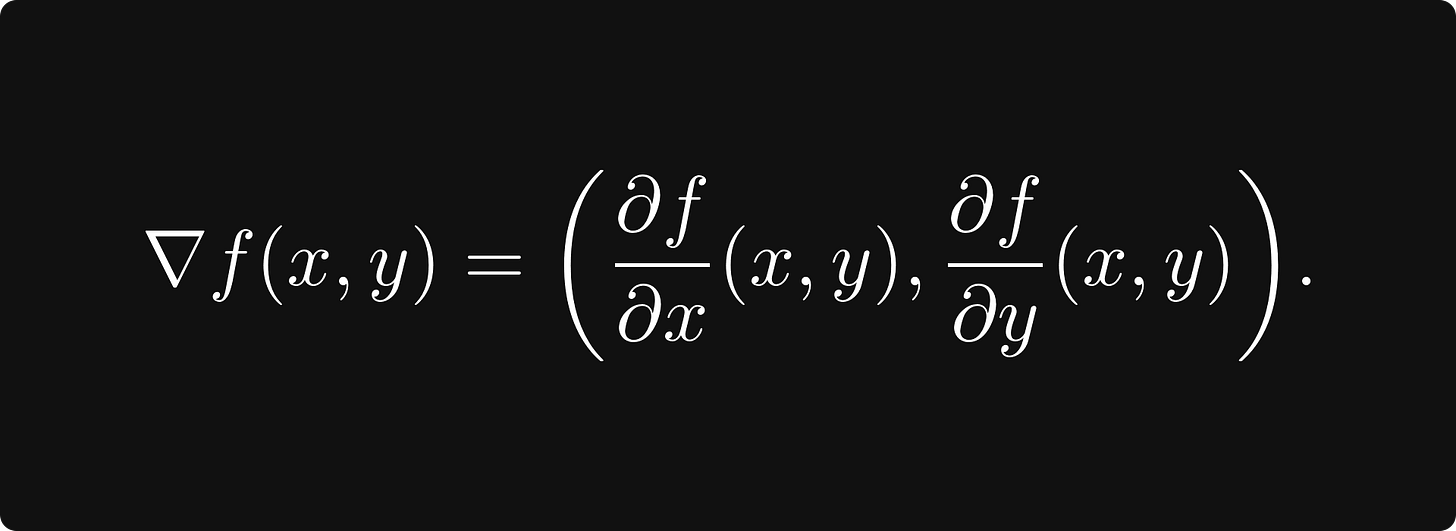
The direction of steepest ascent is given by the gradient, defined by
(Note that the gradient is a direction in the parameter space.)
To summarize, the peak finding algorithm is now
which is called gradient ascent. To find the minimum of a function, we take a step in the direction of the negative gradient, which is the direction of steepest descent:
This version is called gradient descent. You have probably seen this one more frequently since we want to minimize the loss in machine learning.
Why does the gradient point to the steepest ascent?
In this setting, it is not trivial why the gradient gives us the direction of the steepest ascent. To provide an explanation, we need to do some mathematics. Besides slicing the surface with vertical planes perpendicular to the x or y axes, we can slice it with a vertical plane given by any direction (e₁, e₂). With the partial derivatives, we had
We can think about these as derivatives of f(x, y) along the directions (1, 0) and (0, 1). Although these directions are of special significance, we can do this in any direction.
Say, we have the direction e = (e₁, e₂). Then, the directional derivative with respect to e is defined by
Note that the last identity is the dot product of the direction e and the gradient ∇f:
Which direction maximizes the directional derivative? This would be the direction of the steepest ascent, so if we want to optimize, we want to know this particular direction.
To see that this is nothing else than the gradient itself, as we have mentioned, recall that we can write the dot product as
where | · | denotes the length of a vector, and α is the angle between the two vectors. (This is true in an arbitrary number of dimensions, not just in two dimensions.)
This expression is maximized when cos(α) = 1; that is, α is zero, meaning that the vectors e and ∇f have the same direction.
Training neural networks
Now, we are ready to move from theory to practice and see how to train neural networks. Suppose that our task is to classify n-dimensional feature vectors into c classes. To mathematically formalize this, let the function f: ℝⁿ → ℝᶜ represent our neural network, mapping the n-dimensional feature space to the c-dimensional space.
The neural network itself is a parameterized function; we denote its parameters with a single m-dimensional vector w ∈ ℝᵐ. (It is customary to write f(x, w) to explicitly express dependence on parameters.)
Training a neural network is equivalent to finding the minimum of the loss function
J: ℝᵐ → ℝ, mapping the space of neural network parameters to real numbers. The loss function takes the form
where the x-es are the data points with y-s as observations, and L is the term-wise loss that measures the error between the prediction f(x) and the ground truth y.
For instance, if J is the cross-entropy loss, then
where
This might seem innocent enough, but it can be challenging to compute. In real life, the number of data points can be in the millions, so can the number of parameters. So, we have a sum with millions of terms, for which we need to calculate millions of derivatives to minimize. How can we solve this problem in practice?
Stochastic gradient descent
To use gradient descent, we have to calculate
where the expected value is taken with respect to the empirical probability distribution given our training data. We can treat the sequence L(f(xᵢ, w), yᵢ) as independent, identically distributed random variables.
According to the Law of Large Numbers,
holds, where the limit expected value is taken with respect to the true underlying probability distribution of the data. (Which is unknown.)
This means that as we increase our training data, our loss function converges to the true loss. As a consequence, if we subsample our data and only calculate the gradient
for some i instead of all, we still obtain a reasonable estimate if we compute enough.
This is called stochastic gradient descent, or SGD in short, which is by far the most popular optimizer in deep learning. Almost all feasible methods originate from SGD.
Three fundamental developments enable us to effectively train deep neural networks: utilizing GPU-s as a general-purpose computing tool, backpropagation, and stochastic gradient descent. Without SGD, wide adoption of deep learning would not have been possible.
As with almost every new approach, SGD also introduces a whole new can of worms. The obvious question is, how large should our subsample size be? A size that is too small might result in a noisy gradient estimation, while a size that is too large has diminishing returns. Selecting the subsample also needs to happen with care. For example, if all the subsamples belong to one class, the estimate will probably be off by a mile. However, experimentation and proper data randomization can solve these issues in practice.
Improving gradient descent
Gradient descent (with the SGD variant as well) suffers from several issues which can make them ineffective under some circumstances. For instance, as we have seen, the learning rate controls the step size we will take in the direction of the gradient. Generally, we can make two mistakes regarding this parameter. First, we can make the step too large, so the loss fails to converge and might even diverge. Second, we might never arrive at a local minimum because we go too slow if the step is too small. To demonstrate this issue, let's take a look at a simple example and study the function
f(x) = x + 2 · sin(x).
Suppose that we start the gradient descent from x₀ = 2.5, with learning rates
α = 1, α = 0.1, and α = 0.01.
It might not be obvious what is happening here, so let's plot the x-s for each learning rate.
For α = 1, the sequence oscillates between two points, failing to converge to the local minimum. For α = 0.01, the convergence seems to be very slow. However, α = 0.1 seems just right. How do you determine this in a general setting? Their main idea is that the learning rate does not necessarily have to be constant. Heuristically, if the magnitude of the gradient itself is large, we should reduce the learning rate to avoid jumping too far. On the other hand, if the magnitude is small, it probably means that we are getting close to a local optimum, so to avoid overshooting, the learning rate definitely shouldn't be increased. Algorithms changing the learning rate dynamically are called adaptive.
One of the most famous examples of such an adaptive algorithm is AdaGrad. It cumulatively stores gradient magnitude and scales the learning rate with respect to that. AdaGrad defines an accumulation variable $r_0 = 0$ and updates it with the rule
where
denotes the componentwise product of two vectors. This is then used to scale the learning rate:
where δ is a small number for numerical stability, and the square root is taken componentwise. First, when the gradient is large, the accumulation variable grows fast, thus decreasing the learning rate. When the parameter is near a local minimum, gradients get smaller, so the learning rate stops practically.
Of course, AdaGrad is one possible solution to this problem. More and more advanced optimization algorithms are available every year, solving a wide range of issues related to gradient descent. However, tuning the learning rate is beneficial even with the most advanced optimization methods.
Regarding issues with gradient descent, another is, for instance, to make sure that we find a global optimum or a local optimum close to it in value. As you can see in the previous example, gradient descent often gets stuck in a bad local optimum. To get a detailed understanding of the solution for this and the other issues, I recommend reading through Chapter 8 of the Deep Learning textbook by Ian Goodfellow, Yoshua Bengio, and Aaron Courville.
How does the loss function for deep neural networks look like?
In our examples during the previous sections, we have only visualized toy examples like f(x) = 25 · sin(x) - x². There is a reason for this: plotting a function is not straightforward for more than two variables. Since our inherent limitations, we can only see and think in at most three dimensions. However, we are smart, thus, we can employ several tricks to grasp the loss function of a neural network. One excellent paper about this is Visualizing the Loss Landscape of Neural Nets by Hao Li et al., who were able to visualize the loss function by essentially choosing two random directions and plotting the two-variable function
f(a, b) = L(w + au + bv)
(To avoid distortions by scale invariance, they also introduced some normalizing factors for the random directions.) Their investigations revealed how skip connections in ResNet architectures shape the loss landscape, making it easier to optimize.

Regardless of the significant improvement made by skip connections, my point was to demonstrate that highly multidimensional optimization is hard. By looking at the first part of the figure, we see many local minima, sharp peaks, plateaus, and so on. Good architecture design can make the job of optimizers easier, but with thoughtful optimization practices, we can tackle more complicated loss landscapes. These go hand in hand.
Conclusion
In the previous sections, we have learned the intuition behind gradients and defined them in a mathematically precise way. We have seen that for any differentiable function, no matter the number of variables, the gradient always points towards the steepest ascent, which is the foundation of the gradient descent algorithm. Although conceptually very simple, it has significant computational difficulties when applied to functions with millions of variables. This problem is alleviated by stochastic gradient descent. However, there are many more issues: getting stuck in a local optimum, selecting the learning rate, etc. Because of these issues, optimization is hard and requires attention from both researchers and practitioners. There is a very active community out there, making it constantly better with amazing results! After understanding the mathematical foundations of optimization for deep learning, you are on the right path to improving state-of-the-art! Some excellent papers to get you started:
Visualizing the Loss Landscape of Neural Nets by Hao Li, Zheng Xu, Gavin Taylor, Christoph Studer, and Tom Goldstein
Adam: A Method for Stochastic Optimization by Diederik P. Kingma and Jimmy Ba
Calibrating the Adaptive Learning Rate to Improve Convergence of ADAM by Qianqian Tong, Guannan Liang and Jinbo Bi
On the Variance of the Adaptive Learning Rate and Beyond by Liyuan Liu, Haoming Jiang, Pengcheng He, Weizhu Chen, Xiaodong Liu, Jianfeng Gao, and Jiawei Han
The most common optimizers in deep learning
In practical scenarios, there are a optimization methods that perform extremely well. If you would like to do some research on your own, here is a list of references.
Adadelta: ADADELTA: An Adaptive Learning Rate Method by Matthew D. Zeiler
AdaGrad: Adaptive Subgradient Methods for Online Learning and Stochastic Optimization by John Duchi, Elad Hazan, and Yoram Singer
Adam: Adam: A Method for Stochastic Optimization by Diederik P. Kingma and Jimmy Ba
AdamW: Decoupled Weight Decay Regularization by Ilya Loshchilov and Frank Hutter
Averaged Stochastic Gradient Descent: Acceleration of stochastic approximation by averaging by B. T. Polyak and A. B. Juditsky
FTRL, or Follow The Regularized Leader: Ad Click Prediction: a View from the Trenches by H. Brendan McMahan et al.
Lookahead: Lookahead Optimizer: ksteps forward, 1 step back by Michael R. Zhang, James Lucas, Geoffrey Hinton, and Jimmy Ba
NAdam: Incorporating Nesterov Momentum into Adam by Timothy Dozat
RAdam, or Rectified Adam: On the Variance of the Adaptive Learning Rate and Beyond by Liyuan Liu, Haoming Jiang, Pengcheng He, Weizhu Chen, Xiaodong Liu, Jianfeng Gao, and Jiawei Han
Ranger: Ranger21: a synergistic deep learning optimizer by Less Wright and Nestor Demeure
Stochastic Gradient Descent with momentum: On the importance of initialization and momentum in deep learning by Ilya Sutskever, James Martens, George Dahl, and Geoffrey Hinton


