

Discover more from The Palindrome
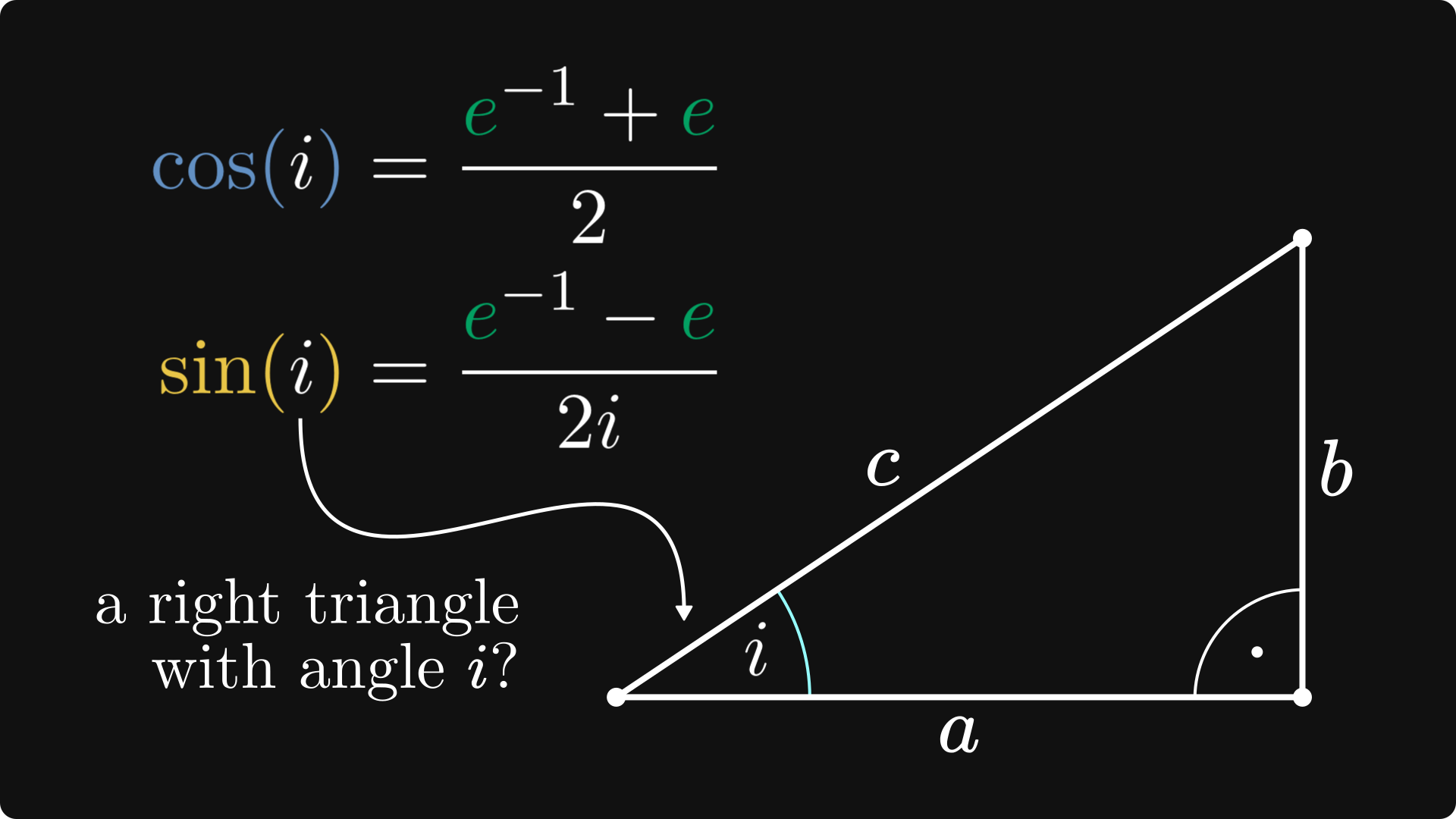
This is not a trick: the cosine of the imaginary number i is (e⁻¹ + e)/2.
How on Earth does this follow from the definition of the cosine? No matter how hard you try, you cannot construct a right triangle with an angle i. What kind of sorcery is this?
Behind the scenes, sine and cosine are much more than a simple ratio of sides. They are the building blocks of science and engineering, and we can extend them from angles of right triangles to arbitrary complex numbers.
In this post, we’ll undertake this journey.
Right triangles and their sides
The history of trigonometric functions goes back almost two thousand years. In their original form, as we first encounter them in school, sine and cosine are defined in terms of right triangles.
For an acute angle α, its sine is defined by the ratio of the opposite leg’s and the hypotenuse’s length. (Where α is an angle in a right triangle.) Similarly, the cosine of α is the ratio of the adjacent leg’s and the hypotenuse’s length.
Even though the sine and cosine formally depend on the sides, they remain invariant to translating, scaling, rotating, and reflecting the triangle.
In other words, the trigonometric functions are invariant to similarity transformations. Thus, sine and cosine are well-defined: they depend only on the angle α.
Because of this, basic trigonometry is used to measure distances. Imagine a lighthouse towering in the distance. If we know its height and measure its angular distance, we can calculate how far the top of the tower is from us using sine and the Pythagorean theorem.
Extension to all angles
What about angles larger than π/2 radians? (Or 90°. But radians are infinitely cooler.) In this case, there is no right triangle, no hypotenuse, and no legs either.
We can find the answer by giving a clever representation of the trigonometric functions. If we move over to the Cartesian coordinate system, we can form a right triangle such that
its hypotenuse is a unit vector,
and its legs are parallel to the x and y axes respectively.
Take a look at this below.
This way, the cosine and sine coincide with the x and y coordinates of our unit vector serving as the hypotenuse. Why is this good for us?
Because we can talk about obtuse and reflex angles! (That is, angles larger than π/2 radians.)
We can also wind our unit vector clockwise to define the sine and cosine for negative angles.
Finally, the definition for an arbitrary real α is complete if we consider that by winding the unit vector around, we can extend the trigonometric functions by periodicity.
Thus, we get the familiar wave-like graphs. Here are sine and cosine, in their (partially) complete glory.
Computing the trigonometric functions in practice
It’s great that we have defined sine and cosine for arbitrary real numbers, but there is one glaring issue: how can we calculate its value in practice?
For certain values, like π/4, we can explicitly construct a corresponding right angle and calculate the ratios by hand.
However, we can’t do this for any α. What to do then? Enter the Taylor polynomials.
The Taylor polynomials
Let’s go back to square one: differentiation. By definition, the derivative of a real function describes the slope of the tangent line at the given point.
By knowing the derivative, we can write the equation for the tangent line.
Again, why is this good? Because locally we can replace our function with a linear one, and linear functions are easy to compute!
In fact, this is the best possible linear approximation. Can we do a better job with higher-degree polynomials?
Yes! It turns out that with the first n-th order derivatives, we can explicitly construct the best approximating polynomial of n-th degree.
This is called the n-th Taylor polynomial.
It gets even better: certain infinitely differentiable functions are exactly reproduced by letting the degree to infinity.
This is called the Taylor series. (Also called a power series.) The question: does this help us calculate the sine and cosine?
Yes, big time.
The Taylor expansion of sine and cosine
I’ll unveil the mystery without further ado: sine and cosine are reconstructed by their Taylor series. (Showing the convergence of a function series is not a trivial matter, so we’ll skip this here.) Thus, to obtain these functions in an infinite series form, we need to compute its n-th order derivatives at zero.
As sine and cosine are the derivatives of each other (up to a factor of -1), we have a simple job.
Moreover, the derivatives are straightforward to evaluate at 0. (Just think of the unit circle definition.) Thus, we obtain the following Taylor expansions.
In practice, we compute finitely many terms, replacing the function with a polynomial. The higher the cutoff point, the better the approximation. By plotting its Taylor polynomials along with the sine function, we see how the approximations eventually smooth over the original function.
The complex trigonometric function
Now that we have a Taylor series representation, can’t we just plug in a complex number? After all, we can raise any complex number to any integer power, so nothing stands in our way.
And thus, extending the trigonometric functions to the complex plane comes for free using the Taylor series. (Well, almost free. We skipped the crazy amount of work needed to make function series mathematically precise.)
Sounds simple enough. Is it useful? Yes. Let me show you the single most mind-blowing connection in mathematics: expressing the exponential function in terms of sine and cosine.
Euler’s formula
The Taylor series is like a Swiss army knife in mathematics. It’s not just for the sine and cosine; a lot of the important functions have a convergent Taylor series representation. (Of course, they are important precisely because they have a convergent Taylor series representation. )
One such function is the famous exponential function. By applying the same process as before, we can find the power series of exp.
Besides the already discussed computational advantages, there is another one. And quite a surprising one to say the least!
By plugging in iz to the power series of the exponential function, a brief but tedious calculation gives us an unbelievable result:
This is the famous Euler’s formula, connecting the complex exponential to trigonometric functions. (The original Euler’s formula is restricted to real numbers, but we’ll let this slide.)
With a bit of algebra, we can express sin and cos in terms of the exponential.
Again, by plugging in z = i here, we show what was hinted at the beginning: the cosine of the imaginary unit i is (e⁻¹ + e)/2.
The polar representation
Euler’s formula is behind the polar representation of complex numbers. Previously, we have seen that the vector (cos(t), sin(t)) parametrizes the unit circle. Thus, by restricting Euler’s formula to the real numbers, we obtain the unit circle.
Any complex number can be described by its absolute value and its phase. (This is an alternative to the default representation provided by the real and imaginary units.) Combining this with Euler’s formula, we obtain the so-called polar representation of complex numbers.
Why is this useful? Check out how two complex numbers are multiplied.
Now, the same with the polar representation.
The latter one is much more revealing. First, it is much simpler, but there is more. Polar representations provide a clear geometric picture: multiplication of complex numbers is equivalent to stretching and rotation!
That’s a long way from right triangles.
The history of trigonometric functions
Isn't this wrong? cos(i) = cosh(1) = e/2 + 1/(2e) is the correct value.