Logistic regression

(is a classification algorithm)

This post is the next chapter of my upcoming Mathematics of Machine Learning book, available in early access.

New chapters are available for the premium subscribers of The Palindrome as well, but there are 40+ chapters (~500 pages) available exclusively for members of the early access.

---

Regression is cool and all, but let's face it: classification is the real deal. I won't speculate on the distribution of actual problems, but it's safe to say that classification problems take a massive bite out of the cake.

In this chapter, we'll learn and implement our very first classification tool. Consider the problem of predicting whether or not a student will pass an exam given the time spent studying; that is, our independent variable x ∈ ℝ quantifies the number of hours studied, while the dependent variable y ∈ {0, 1} marks if the student has failed (0) or passed (1) the exam.

How can we whip up a classifier that takes a float and conjures a prediction about the success of the exam?

Mathematically speaking, we are looking for a function h(x): ℝ → {0, 1}, where h(x) = 0 means that a student who studied x hours is predicted to fail, while h(x) = 1 predicts a pass. Again, two key design choices determine our machine learning model:

• the family of functions we pick our h from (that is, our hypothesis space),

• and the measure of fit. (That is, our loss function.)

There are several avenues to take. For one, we could look for a function h(x; c) of a single variable x and a real parameter c, defined by

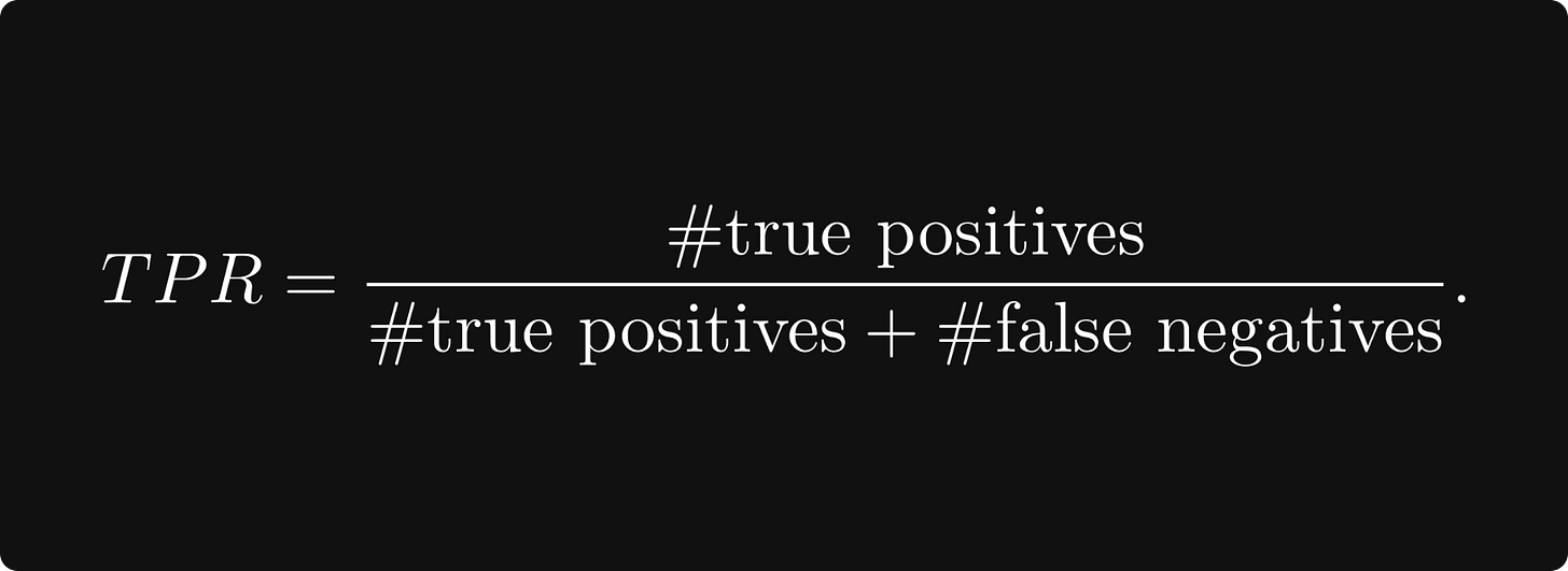
then find the c that maximizes the true positive rate

This avenue would lead us to decision trees, a simple, beautiful, and extremely powerful family of algorithms routinely beating Starfleet-class deep learning models on tabular datasets. We'll travel this road later on our journey. For now, we'll take another junction, the one towards logistic regression. Yes, you read correctly. Logistic regression. Despite its name, it's actually a binary classification algorithm.

Let's see what it is!

The logistic regression model

One of the most useful principles of problem solving: generalizing the problem sometimes yields a simpler solution.

We can apply this principle by noticing that the labels 0 (fail) and 1 (pass) can be viewed as probabilities. Instead of predicting a mere class label, let's estimate the probability of passing the exam! In other words, we are looking for a function
h(x): ℝ → [0, 1], whose output we interpret as

(In yet another words, we are performing a regression on probabilities.)

---

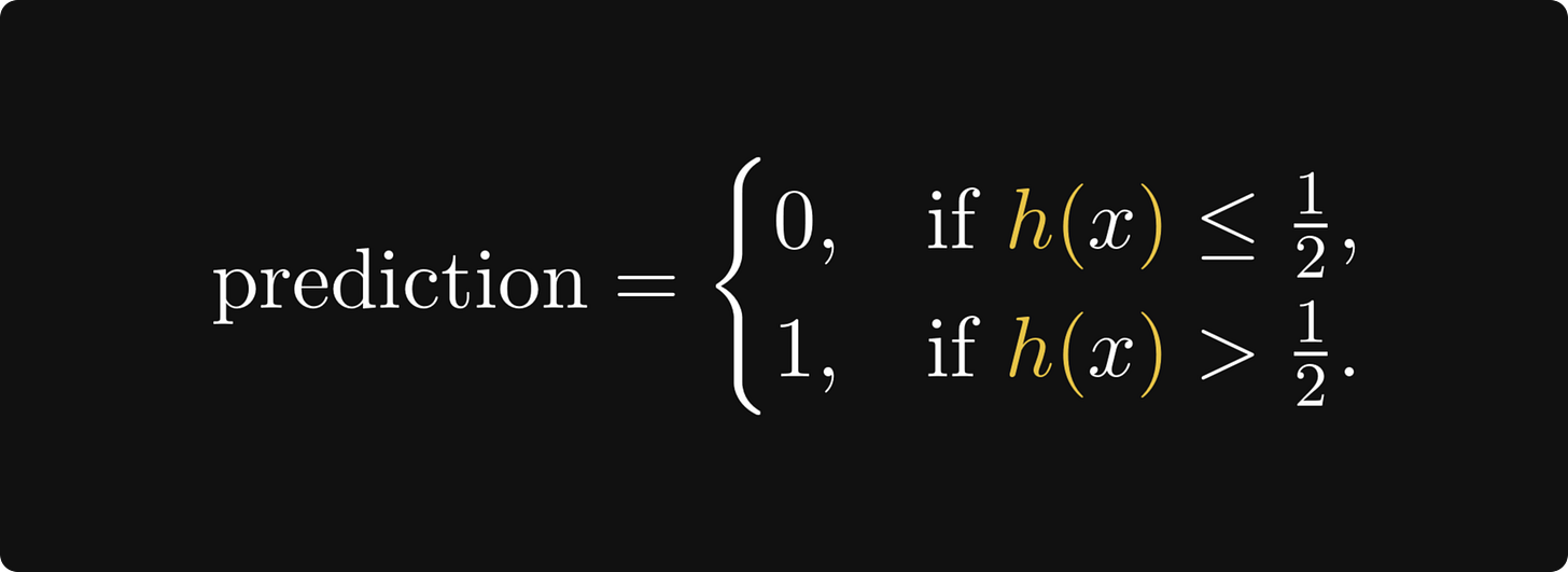
Remark. (The decision cut-off.) Sometimes, we want to be stricter or looser with our decisions. In general, our prediction can be

for the cut-off c ∈ [0, 1]. Intuitively speaking, the higher c is, the more evidence we require for a positive classification. For instance, when building a skin cancer detector, we want to be as certain as possible before giving a positive diagnosis. (See the Decision Theory chapter of Christopher Bishop’s book Pattern Recognition and Machine Learning for more on this topic.)

---

The simplest way to turn a real number - like the number of study hours - is to apply the sigmoid function

Here is its NumPy implementation.

def sigmoid(x):
  return 1/(1 + np.exp(-x))

Let's see what we are talking about.

The behavior of sigmoid is straight-forward:

From the perspective of binary classification, this can be translated to

• predicting 0 if x ≤ 0,

• and predicting 1 if x > 0.

In yet another words, 0 is the decision boundary of the simple model σ(x). Can we parametrize the sigmoid to learn the decision boundary for our fail-or-pass binary classification problem?

A natural idea is to look for a function h(x) = σ(ax + b). You can think about this as

1. turning the study hours feature x into a score ax + b that quantifies the effect of x on the result of the exam,

2. then turning the score ax + b into a probability σ(ax + b).

(The model h(x) = σ(ax + b) is called logistic regression because the term "logistic function" is an alias for the sigmoid, and we are performing a regression on probabilities.)

Let's analyze h(x).

def h(x, a, b):
    return sigmoid(a*x + b)

Geometrically speaking, the regression coefficient a is responsible for how fast the probability shifts from 0 to 1, while the intercept b controls where it happens. To illustrate, let's vary a and fix b.

Similarly, we can fix a and vary b.

So, we finally have a hypothesis space

How can we find the single function that fits our data best?