Linear regression in multiple variables

(finally) entering higher dimensions

Hi there! This post is from my upcoming Mathematics of Machine Learning book, available in early access.

New chapters are available for the premium subscribers of The Palindrome as well, but there are 40+ chapters (~500 pages) available exclusively for members of the early access.

---

So far, we've studied and implemented two machine learning algorithms: linear and logistic regression in a single lonely variable. As always, there's a hiccup. Real datasets contain way more than one feature. (And they are rarely linear. But we'll cross that bridge later.)

In this chapter, we'll take one step towards reality and learn how to handle multiple variables.

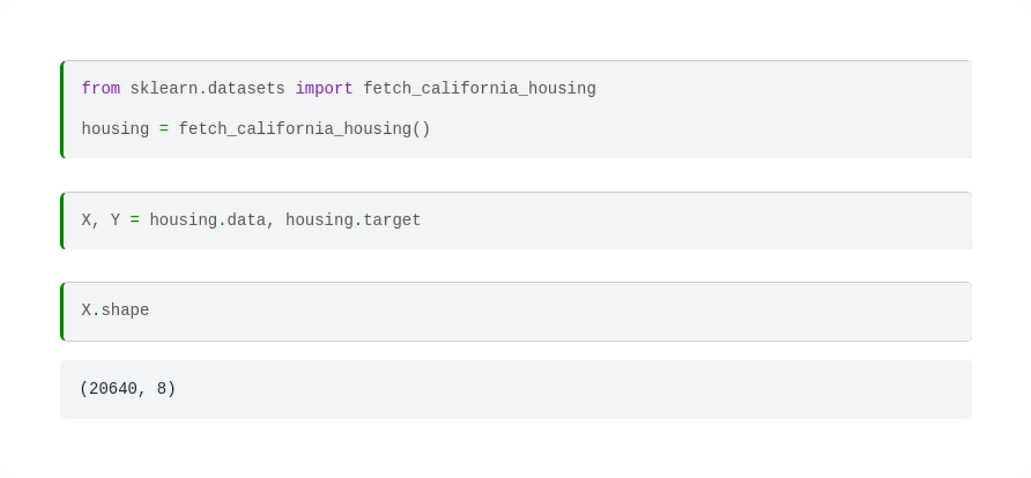
First, look at the famous California housing dataset from scikit-learn. The dataset holds of 20640 instances, each consisting of

• a vector x ∈ ℝ⁸ of 8 features describing a census block group (such as median income per block, the average number of rooms per household, etc.),

• and a target variable y ∈ ℝ, containing the median house value for the census block group.

The housing object contains two NumPy arrays: the data and the target. Let's unpack them and check their shape!

As the shape (20640, 8) indicates, each row of the matrix X represents a data sample, and each column corresponds to a feature. Here's a data sample:

Mathematically speaking, each data sample is a row vector, and each feature is a column vector.

---

Remark. (The eternal dilemma of row vs column vectors.)

You might have noticed that while data samples come in row vectors, we've used column vectors throughout our entire study of multivariable functions. Both choices are properly justified: column vectors are convenient for theory, but row vectors are perfect for practice.

To make this extremely (and often redundantly) clear, we'll indicate this by using the matrix notation ℝ¹ ˣ ᵐ for row vectors and ℝⁿ ˣ ¹ for column vectors.

(However, to lean towards practice, we'll prefer row vectors from now on.)

---

On the other hand, the ground truths for the target variable are stored in a massive row vector, represented by the NumPy array Y of shape (20640, ).

To predict the median house value y ∈ ℝ from the feature vector x ∈ ℝ⁸, we'll use machine learning. (Surprise.) Mathematically speaking, we are looking for a regression model in the form of a multivariable function f : ℝ⁸ → ℝ. Practically speaking, our task is to construct a function that maps an array of shape (8, ) into a float.

You all know me well by now: minimizing complexity is one of my guiding principles. So, let's build a model that is useful and dead simple at the same time. What's our very first idea when we hear the term "simple"?

Linear regression.

The generalization of linear regression

Recall that for a single numerical feature x ∈ ℝ, the simplest regression model was the linear one; that is, a function of the form h(x) = ax + b for some a, b ∈ ℝ. Intuitively speaking, a quantified the effect of the feature x on the target variable y, while b quantified the bias.

A straightforward generalization is the model

where

• x = (x₁, …, x_d) ∈ ℝ¹ ˣ ᵐ is a d-dimensional feature vector,

• a = (a₁, …, a_d) ∈ ℝ¹ ˣ ᵈ is the regression coefficient vector,

• b ∈ ℝ is the bias,

• and w = (a₁, …, a_d, b) ∈ ℝ¹ ˣ ⁽ᵈ⁺¹⁾ is the vector of parameters.

Author’s note: much to my surprise, Unicode doesn’t contain a subscript version for the character “d”. Because of this, I denoted the symbol “a sub d” by a_d. Apologies!

For a given parameter configuration, h(x) determines a d-dimensional plane. It's simpler to visualize a two-variable example. Here's a NumPy implementation of a simple linear model with coefficients a₁ = 0.8, a₂ = 1.5, and b = 3.