How large that number in the Law of Large Numbers is?
All large numbers are large, but some are larger than others
Today’s issue is a collaboration with Levi from Data Ground Up. He’s been one of my favorite explainers lately, and this post grew out of our recent discussion about the law of large numbers. Enjoy!
Large numbers != large numbers.
Is 100 large? It depends. Do we compare it to 0.001 or 100000? Just like a lot of things in life, the term "large" is relative.
In this post, we explain how large "large" is and prove why you are (probably) wrong about the LLN.
The Law of Large Numbers (LLN)
Let's run an experiment: we’ll roll a dice, just like we did in our introductory probability classes. We keep going until thousands of rolls, calculating the average of the tosses every time.
(Keep in mind that the expected value of a dice roll is (1+2+3+4+5+6)/6 = 3.5.)
Here are the first 10 rolls visualized.
First, we rolled a 5, then we rolled a 1, and so on.
Now let's see what happens if the number of experiments are increased to 100 and 1000:
The "larger" our number is, the closer the sample averages are to the true expected value. The law of large numbers states precisely this: the sample average converges to the expected value.
If we want to be more precise, there are two versions of the law of large numbers: weak and strong.
The weak law states the following.
In other words, the probability of the sample average X̅ₙ falling however far from the expected value μ converges to zero as the number of samples (n) grows. (We’ll take a deeper look at this later.)
It seems that n = 1000 is "large" enough in the dice experiment. What about others?
Let’s see another example! Consider this scratch ticket from Texas.
The official webpage states:
Over $829 million in total prizes in this game!
Prizes start at $150!
Chance to win $20,000,000
The ticket costs only $100!
Sounds awesome, but we know math better than being fooled by these numbers. If we dig deep we can find the odds of winning. This is the price table from the official site.
Knowing these we can easily calculate our chance and the expected values:
the chance to win something is 26.34%,
and the expected payoff is $75.28958 per ticket. (Not counting the $100 entry price.)
It seems like it isn't worth buying the ticket for $100, since the expected value is only ~$75.3.
Now let’s run a similar experiment to the dice example. We (hypothetically) buy more and more tickets, computing the average winnings meanwhile. The more tickets we buy, the closer we will be to the expected value ~$75.
We are not so lucky with our first ten tickets.
Let’s buy ninety more! With a hundred tickets we are getting closer, but we want something smooth on the long run around the orange line.
Let’s do a bigger jump: increase n to 10,000.
Now we have the smooth line, but it’s not what we expected at all! It hovers around $67, not the expected value.
Let’s go further. With one million tickets something strange happened again: we got lucky, and the win pulled the average up. Now, we are even further away!
It seems that 1,000,000 is still not a “large” number!
Let’s go further! With ten million tickets we have several bigger wins that pull up the average, but the effect is getting smaller and smaller. Slowly, but we are getting close to the expected value.
Now we finally have the expected smooth line hovering around the true average.
Even though we could illustrate the law of large numbers with a thousand rolls in the first experiment, a million was barely enough in the second.
Large numbers != large numbers.
How can we explain the strange things that happened in the second experiment?
Variance and the speed of convergence
Let’s zoom into the (weak) law of large numbers!
In essence, the probability P(|X̅ₙ - μ| > ε) measures the distance of the sample average from the true average (that is, the expected value) in a probabilistic sense.
The smaller ε is, the larger the probabilistic distance. Mathematically speaking, the following holds.
Now, the weak law of large numbers states that
that is, the probabilistic distance gets as small as we want.
Loosely speaking, this means that the sample average equals the true average plus a distribution that gets more and more concentrated to zero. In other terms, we have
an asymptotic expansion in a distributional sense. The term o(1) indicates a distribution that gets more and more concentrated to zero as n grows. You might be familiar with the small and big O notation; it’s the same but with probability distributions.
Does the weak law of large numbers and our asymptotic expansion explain what happens with our lottery tickets; that is, why do we need ten million samples to get reasonably close to the true average?
The answer is a short and harsh no.
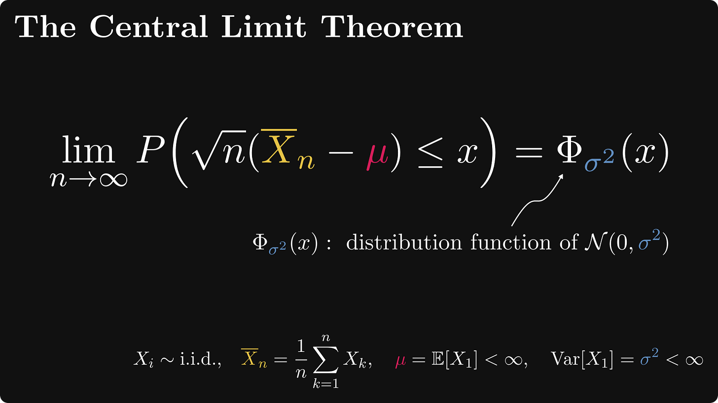
We need a bigger boat asymptotic expansion. Our tool for that is going to be the central limit theorem, one of the most famous results in probability theory, formalizing why the sample averages resemble Gaussian distributions.
The Central Limit Theorem
Let’s dive straight into the deep waters and see the central limit theorem (CLT). It states that in a distributional sense, the √n-scaled centered sample averages converge to the standard normal distribution. (The notion “centered” means that we subtract the expected value.)
To reiterate, convergence holds in a distributional sense. This is just the fancy way of saying that the cumulative distribution functions are pointwise convergent. (I know. Convergences in probability theory are quite convoluted.)
Let’s unpack it: in terms of an asymptotic expansion, the Law of Large Numbers and the Central Limit Theorem imply that
that is, the sample average equals the sum of 1) the expected value μ, 2) a scaled normal distribution, and 3) a distribution that vanishes faster, than 1/√n.
That is, in terms of our asymptotic expansion, we have
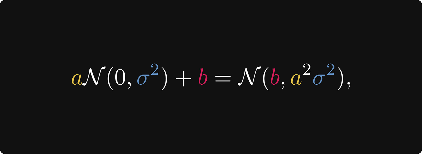
This can be written in a simpler form by amalgamating the constants into the normal distribution. More precisely, we have
meaning that our asymptotic expansion takes the form
In other words, for large n, the sample average approximately equals a normal distribution with variance σ²/n. The larger the n, the smaller the variance; the smaller the variance, the more the normal distribution is concentrated around the expected value μ.
This finally answers our question: how large is that ominous number in the law of large numbers? It depends on the variance of our distribution!
We can read from the asymptotic expansion that if the variance is 10x larger, we need roughly 10x the number of samples for the average to be as close as originally. This is because of the σ²/n term, where σ² represents the variance of our sample X₁, X₂, …, Xₙ, and n represents the number of samples.
Let’s revisit the dice roll and the lottery examples. The variance of a dice roll is 35/12 ≈ 2.916, while the Texas lottery’s variance is approximately 157 000 000. This is a fifty million increase. This means that on average, we’ll need a fifty million times larger sample for the sample average to be as close to the true average as in the case of dice rolls.
It’s important to note that as the law of large numbers is a probabilistic statement, claims like “we need fifty million more samples” are understood probabilistically. If we are lucky, the sample average might be very close to the true average after a few thousand samples.
Conclusion
The law of large numbers is frequently misunderstood.
We use it quite often, but there is an important caveat. Although the sample average (almost surely) converges to the expected value, the speed of the convergence depends on the variance of our sample. The larger the variance, the slower the convergence.
This is bad news for many practical applications. For instance, this is why the convergence of the Monte Carlo method is slow. In a real-life scenario, like gambling, you might even run out of money before you finally start winning. (Though most casino games have a negative expected value, so you’ll always lose on the long run.)
The lesson? Always keep the speed of convergence in mind when applying the law of large numbers.


