Computational Graphs and the Forward Pass

Reverse-engineering the computational graph interface

Now that we understand how to work with computational graphs, it's time to pull back the curtain and see how they work on the inside. After all, this is what we're here for. (At least, it's why I'm writing this.)

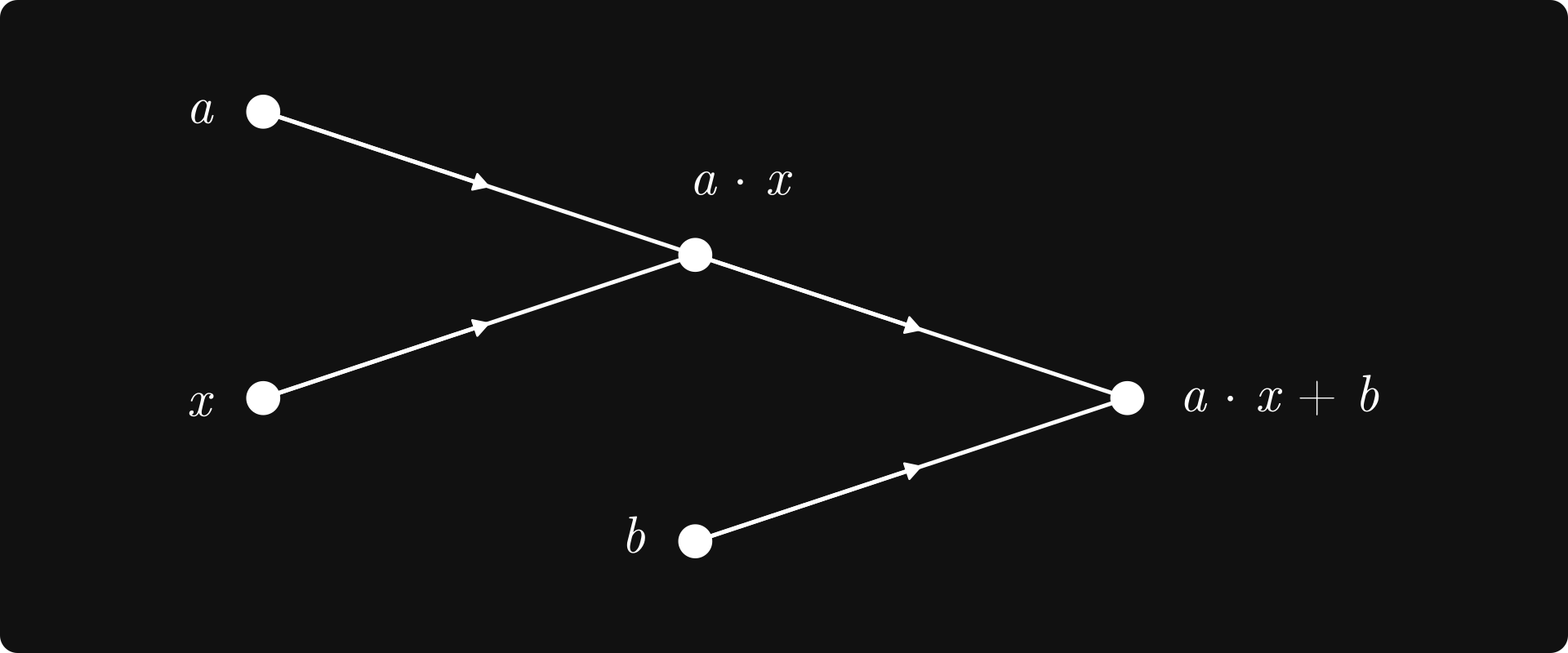
A quick recap: a computational graph is the graph representation of a mathematical computation. By considering the order of operations, we can represent any expression in a graph form. For instance, here's the graph representation of ax + b.

It’s not just linear regression. Any neural network, no matter how large, can be described with a computational graph. Our goal is to implement them from scratch to gain a deep understanding of how they work.

The plan:

• understand how to work with computational graphs,

• and reverse-engineer the implementation.

For this purpose, I have built mlfz, an educational machine learning library, where computational graphs are represented by the Scalar class. You can simply define graphs by using expressions such as y = a * x + b, and compute the gradient

by calling the y.backward() method.

Just like this:

Let’s pop the hood!

---

This post is the third part of my Neural Networks from Scratch series. Although I aim for every post to be self-contained, check out the previous episodes to get you up to speed.

• Episode 1: Introduction to Computational Graphs

• Episode 2: Computational Graphs as Neural Networks

---

The forward pass

As we've seen before, Scalar implements a node in a computational graph. Thus, it must keep track of three attributes:

• a numeric value,

• the backwards gradient,

• and the list of incoming edges.

This chapter progressively implements the Scalar class by adding more and more features. Note that most of the versions here won't have the full functionality of mlfz.nn.scalar.Scalar. The full source can be found on GitHub, but the Python code is not exactly a linear front-to-back text, so we'll unravel it one feature at a time.

(To play around with the code in this post, check out this notebook.)

Here we go:

(I have also added a simple string representation for readability.) Now, we add the meat to the bones. The first thing to do: build the computational graph via operations.

Building the graph

We are already familiar with the Scalar interface: the computational graph is built via applying operations and functions.

How is this done? By overloading the operations using magic methods. In the object oriented Python, there are several of them:

• addition a + b is done via __add__,

• subtraction a - b is via __sub__,

• negation -a is via __neg__,

• multiplication a * b via __mul__,

• division a / b via __truediv__,

• exponentiation a ** b via __pow__,

and many more. I'll do the __add__, you'll do the rest in an exercise. We'll code first, discuss later.

(As this post is written in Jupyter Notebooks, we can iteratively define classes method by method. To avoid writing out all the previously implemented methods each time we add a new one, we inherit the new `Scalar` class from the old one. Keep this in mind, as I'll use this trick later.)

The `__add__` method simply initializes a new `Scalar` instance, formed from the operands. (In this case, `self` and `other`.)

Now, we have a way to track the nodes preceeding z:

Can you implement the rest of the operations? Give them a go before revealing the answer below.

Testing:

Interoperability with Python's number types

At its current state, operations with Python's number types are not supported. Check this out:

The source of this AttributeError is that the expression Scalar(1) + 2 calls Scalar.__add__, with arguments Scalar(1) and 2. As 2 is not a Scalar object, we immediately run into an issue.

How can we solve this? One simple way is to check the Scalar-ness of the second operand, and make the appropriate conversions if needed.

Does it work?

Yes, it does!

Operations, left and right

Now that we've enabled operations with vanilla Python number types, can you guess the output of the expression `2 + Scalar(1)`?

Check this out.

What happened?

In Python, the expression a + b is equivalent to the function call a.__add__(b). In our case, the left operand is a number, and its __add__ method doesn't support Scalars. However, there's another magic method called __radd__, implementing the addition from the left side.

What does that mean? That Python falls back to __radd__ whenever __add__ doesn't work. To be precise, whenever you call a + b,

• a.__add__(b) is called,

• and if it fails, Python attempts to call b.__radd__(a),

• and if it fails as well, a TypeError is thrown.

So, let's add __radd__.

Does it work?

Again, it does!

There are magic methods corresponding to the other operations as well:

• __rmul__,

• __rtruediv__,

• and __rsub__.

Feel free to implement them as an exercise before looking at the answer below:

Testing:

Defining functions for nodes

So far, we've only added support for arithmetic operations such as +, -, *, /, and **. What about functions? After all, machine learning models are defined by mathematical expressions such as f(x) = σ(ax + b), where

is the sigmoid function. How to do that with Scalar instances?

There are multiple potential approaches; we'll go with functions that take and return Scalar objects. This is simpler than you think. Here we go:

In mlfz, these can be found at mlfz.nn.scalar.functional. Nothing fancy, just plain old sin, cos, sigmoid, relu, and other machine learning-related functions.

The analogous implementation of the sigmoid function is below. If you have the chance, give it a go before revealing the solution below.

This works as expected:

Implementing the forward pass

Let's put all of this together and check how the computational graph is built upon applying the operations.

For that, we need a function that recursively traverses all parent nodes and returns the directed graph, using the `Digraph` object from the `graphviz` library.

We'll study the simple computational graph defined by σ(a x + b) + a, where σ(x) is the familiar sigmoid function.

(The above is equivalent to the expression sigmoid(a * x + b) + a, but I choose to break it up into smaller components to assign variables to all intermediate results.)

First, y = a * x + b is computed.

The second step is the application of the sigmoid function, adding a child node to y.

To make things more exciting, we add another node, but this time, we attach it to
s = sigmoid(y) and the input node a = Scalar(0.2).

What we've seen here is the forward pass corresponding to the computational graph of sigmoid(a * x + b) + a: the input nodes a, b, and x are propagated through the graph to calculate the value z = sigmoid(a * x + b) + a, one step at a time.

To train neural networks, we utilize the gradient algorithm that, in turn, requires us to compute the derivative of the final node with respect to all other nodes. This is done in the backward pass, and we'll learn what it is in the next post.