

Understanding k-Nearest Neighbors
Understanding k-Nearest Neighbors
Show me your neighbors, I’ll tell you who you are


How long does it take to train the k-nearest neighbor model?
Zero seconds.
It sounds crazy, but kNN is lazy as hell. This model is not training at all!
The group of supervised learning algorithms is broad, but kNN is an outlier. It is a relatively simple model, so it is a good starting point for beginners. There’s also some beautiful math behind: kNN gives us a way to see the importance of distance metrics — an otherwise abstract concept — in real-life machine-learning scenarios.
On the surface, kNN looks basic, but it is behind advanced (and hyped-up) techniques such as vector similarity search! Whenever you search with an image on Google, there’s (probably) some version of kNN behind.
By the end of this post, you’ll deeply understand how kNN and other lazy algorithms work and why distance is one of the most essential concepts in data science and machine learning.
Let’s dive into it!
This post is a collaboration with my friend
from Data Ground Up. He is well-known for explaining concepts from data science and machine learning. (“Explaining Data Science on Grandma's level“, as he puts it.)We have found kNN to be a worthy topic to discuss: it is simple on the surface but intricately intertwined with deep concepts such as distance and similarity. Enjoy!
How kNN works
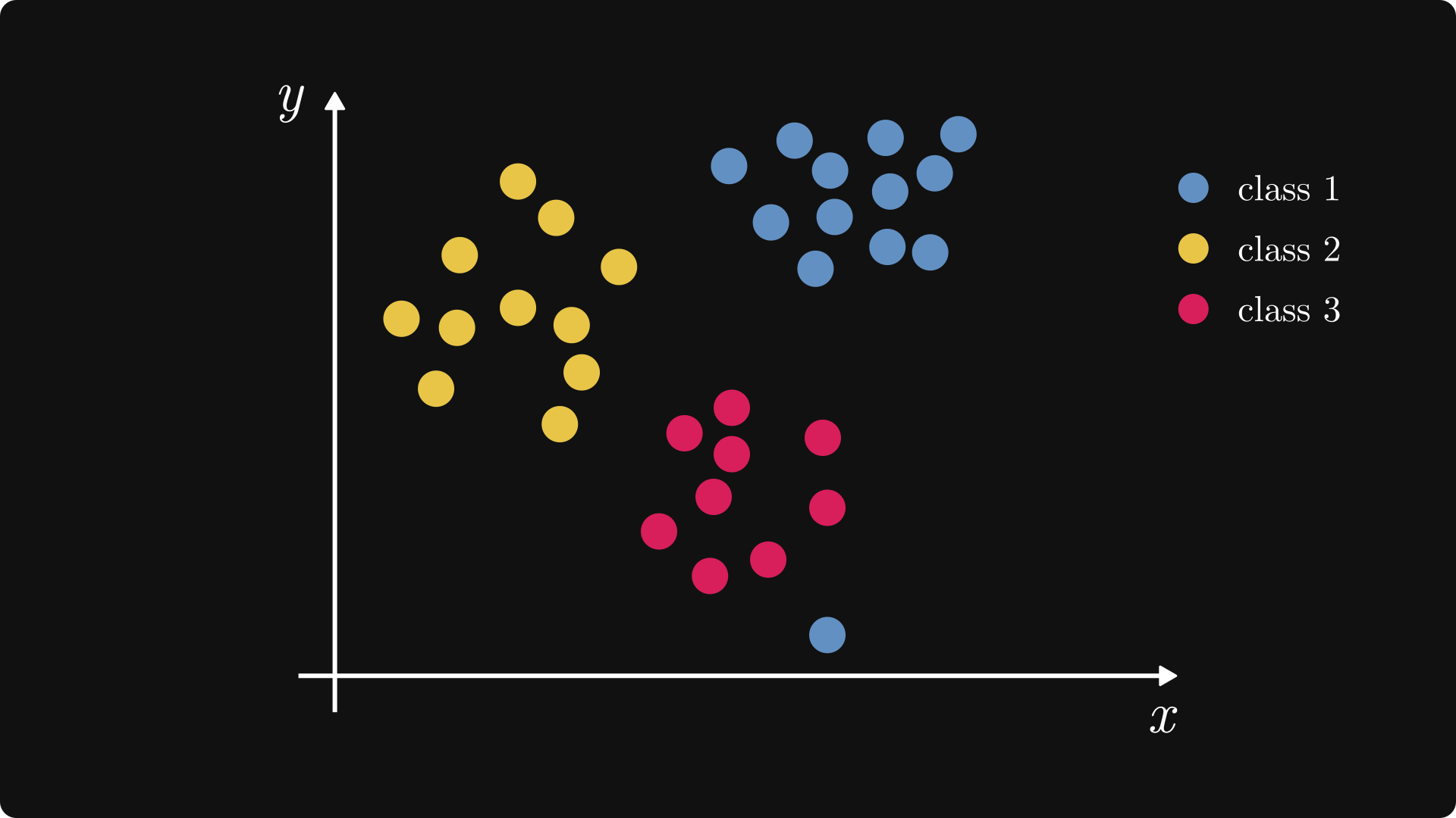
kNN is mainly used for classification, so let's consider the following example.
We’ll use a toy dataset with three categories: Blue, Yellow, Red. Say, each sample represents a document in a vector database, and each class is a category: scientific, literature, or news article.
In machine learning, we use this data to train a generalized model. kNN is an exception: it doesn’t even look at this dataset until a new data point comes in for inference!
That’s why it’s called lazy. Lazy models don’t learn from the training set; instead, they store it and pull it up every time for a prediction.
kNN makes predictions by
calculating the distances between the new sample and the training samples,
finding the k nearest neighbors,
and classifying the new sample via a majority vote from those k nearest neighbors.
In other words, you show kNN your neighbors, and kNN tells who you are.
Words rarely do algorithms justice, so here’s a reference implementation in Python. We’ve even prepared a Jupyter Notebook for you so you can play around as much as you want.
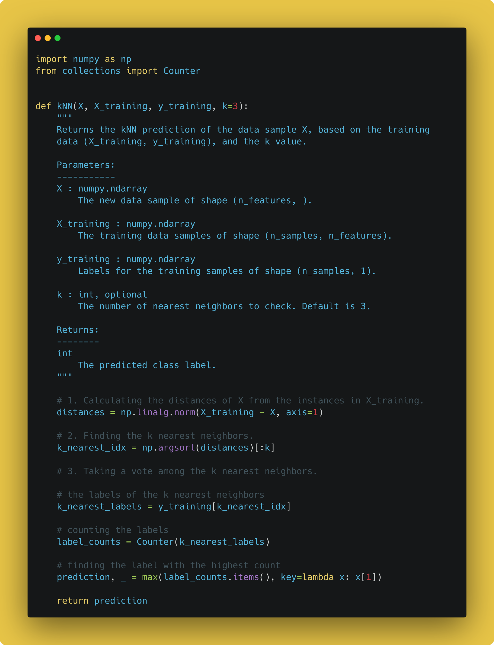
kNN can be used for regression as well: just do an averaging instead of a majority vote in the last step. We’ll stick to classification though. (In any case, implementing the kNN-based regressor is a great exercise.)
The value of k
As you can see from the algorithm, the value of k is really important, as it determines the number of samples we consider for the prediction.
Let's add a new data point that we want to classify and set k = 3. This is what we get.
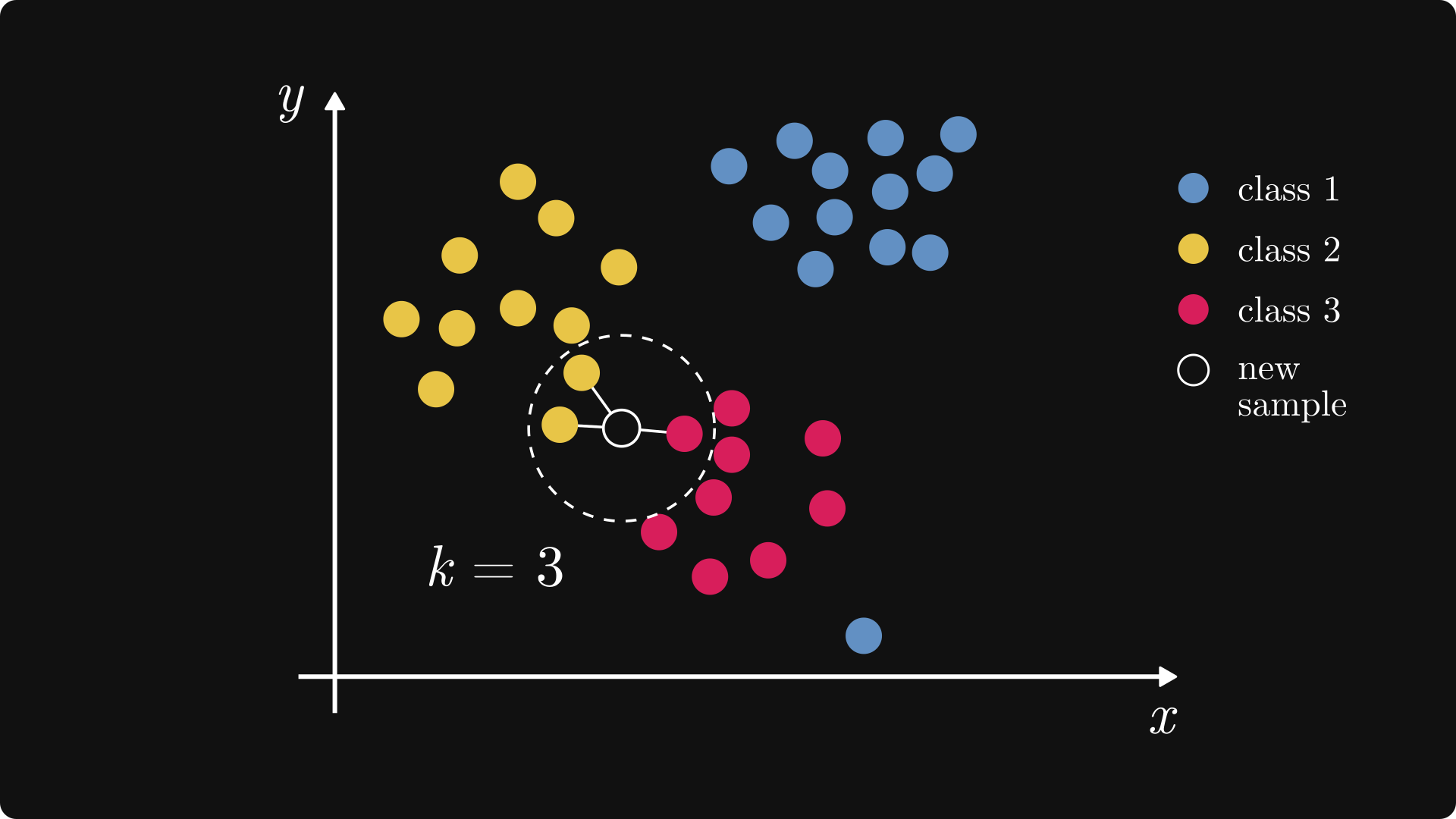
k tells the model: “Let’s consider the k closest samples for prediction.” In this case, the k = 3 closest values are two Yellow and one Red samples. Yellow is dominant, so we predict the new data point Yellow.
The parameter k has a huge effect on the outcome. If we change it to k = 8, the result is totally different.
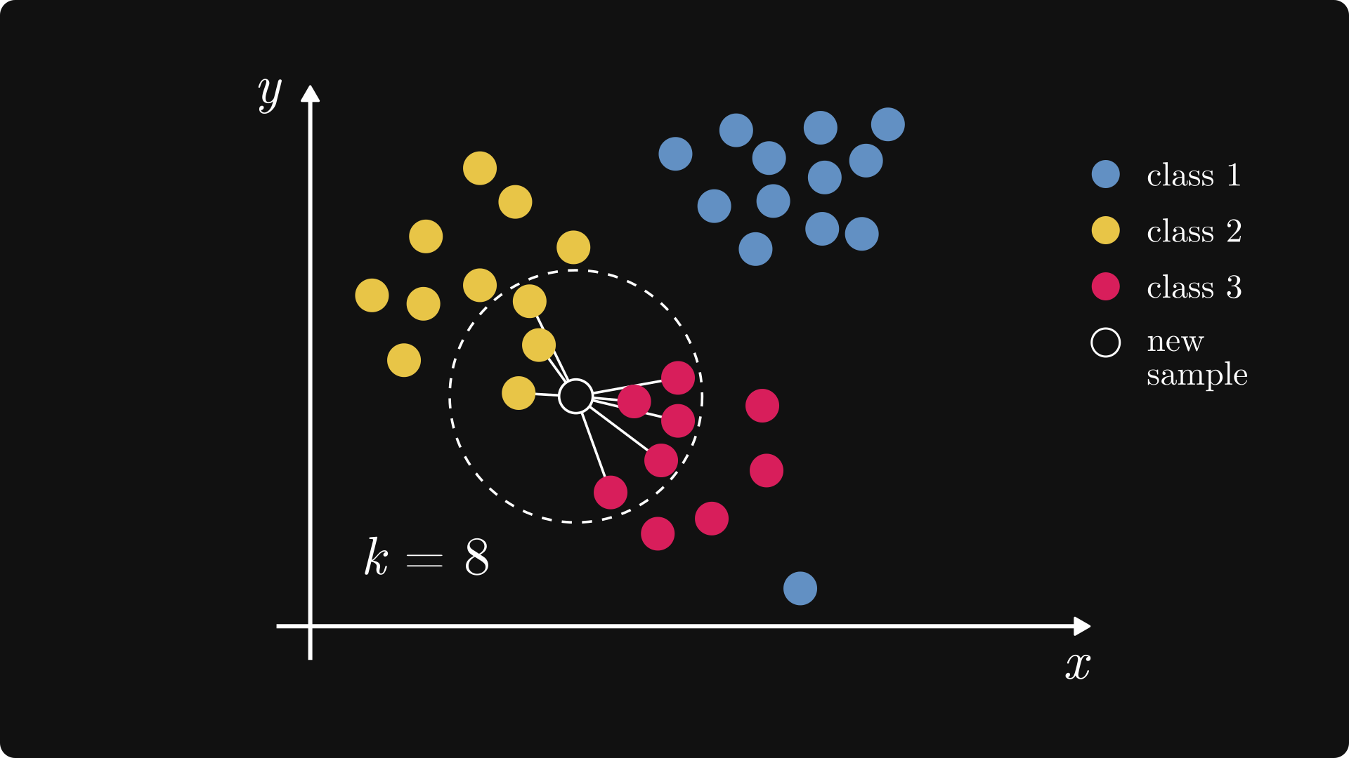
Now, Red has become dominant. Thus, the new sample is predicted to be Red as well.
If we use a small value for k, the model may overfit. Let's introduce an outlier to our data and use k = 1!
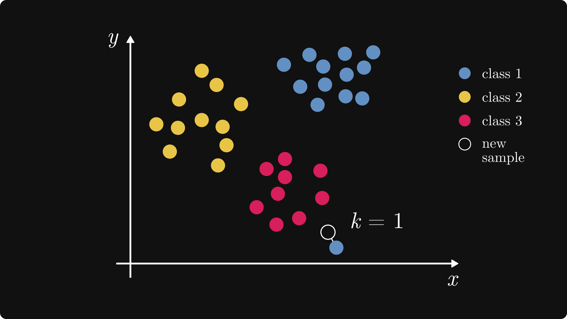
In this case, the closest point to the new data is an outlier, so the new data is probably Red. With a small value of k, the noise has a higher impact.
On the other hand, if k is large, the patterns in the data get averaged out, and the predictions eventually become the most populous class. Thus, the choice of k is a tough one, often done through parameter search. That’s a massive topic on its own.
What if we have an even value as k and two (or even classes)?
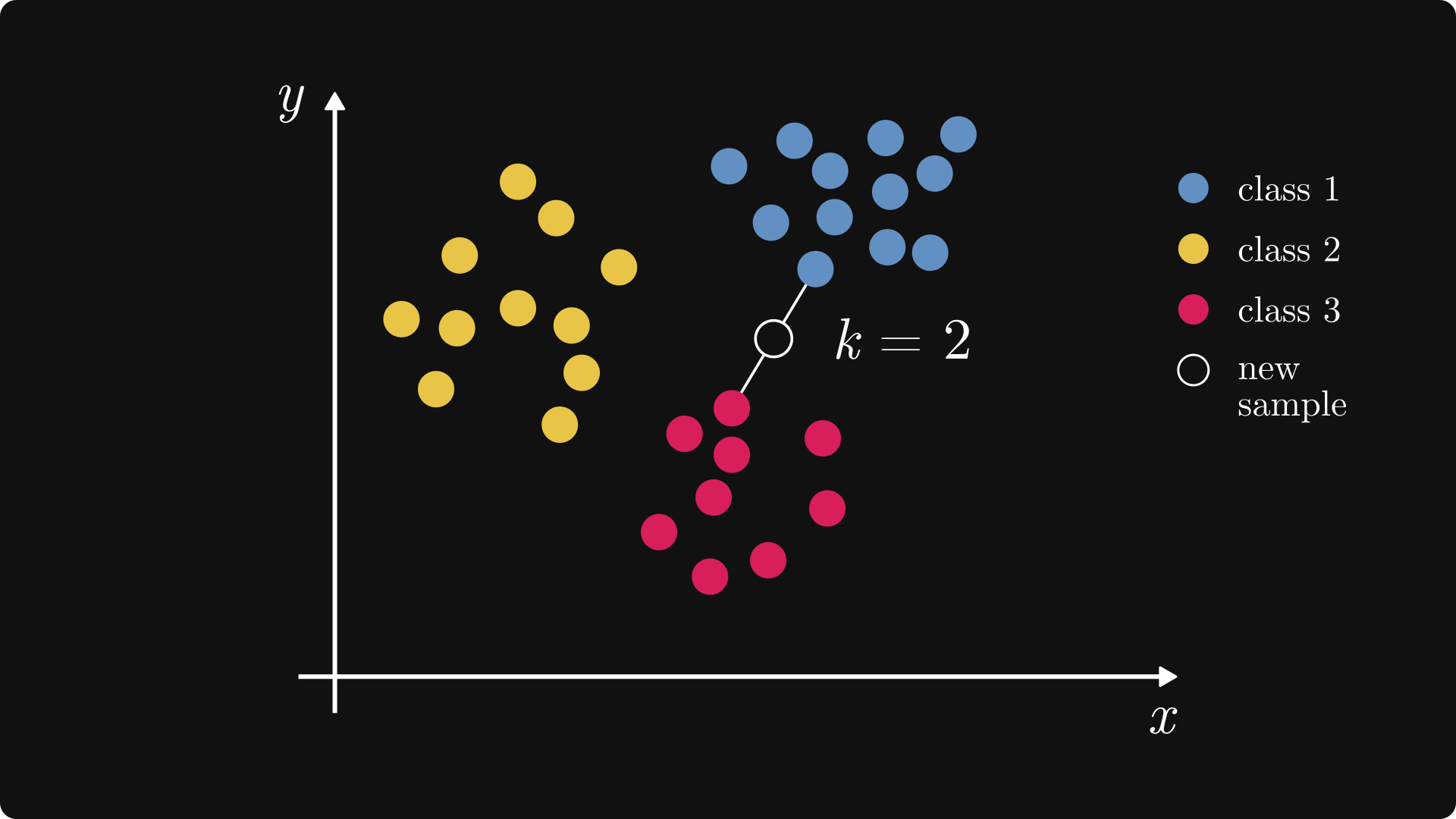
In this example, we cannot choose between Blue and Green. We have two options: Leave the new data unclassified or randomly select between Blue and Green. With even values of k, ties can occur, so it's better to use an odd value.
Another solution to decide ties can be the weighted kNN. The weighted model considers not only the majority vote of the k nearest neighbors but also how far away each one is. The closer the sample, the higher the weight is.
Now that we know everything about k, let’s discuss the other important part of the model: those dashed lines on the illustrations.
Distance metrics
Recall the very first thing that kNN does. We wrote, quote, “calculating the distances between the new sample and the training samples”.
You might notice that something is missing here. What is distance, really? It depends.
In machine learning, we use different distance metrics, depending on the problem. It’s time for mathematics to enter the chat.
Euclidean distance
The Euclidean distance is the most used metric in (almost) every applied and pure field. It is simply the length of the shortest line segment between two points in the space.
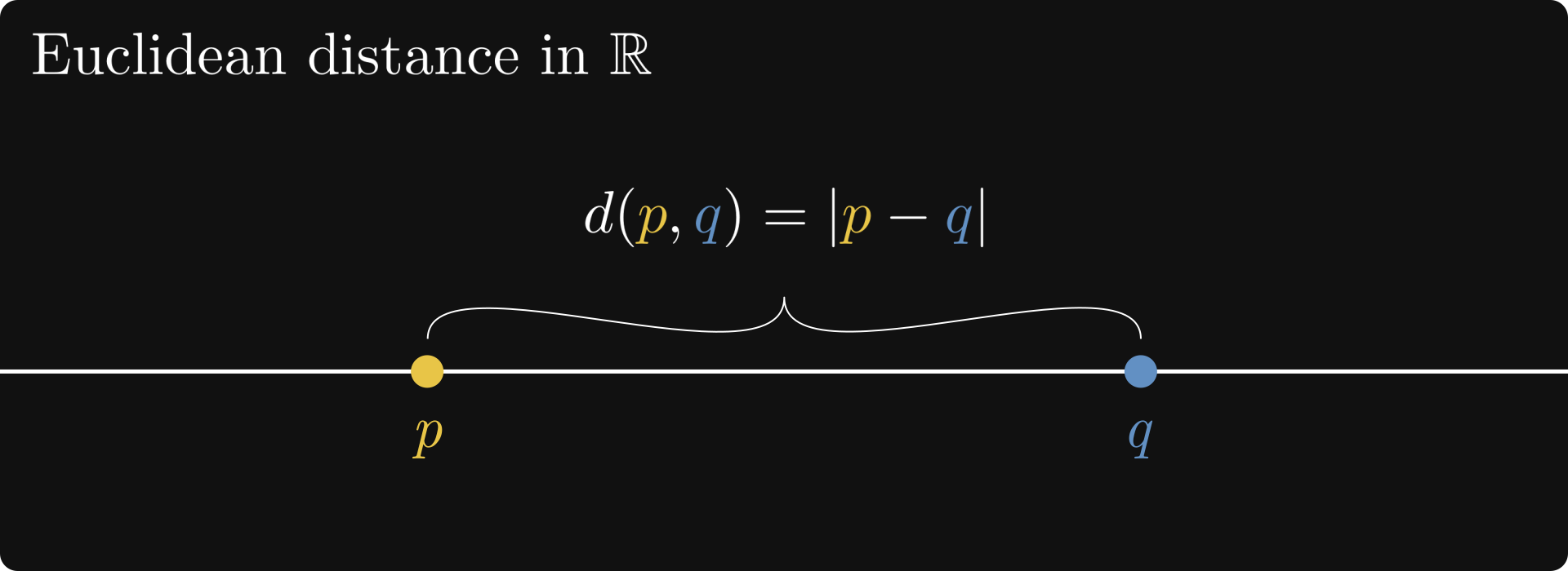
Let’s start in one dimension.
In 1D, the distance between two points on a line is the absolute value of their numerical difference. Mathematically speaking, the Euclidean distance of two points p and q is defined by d(p, q) = |p - q|.
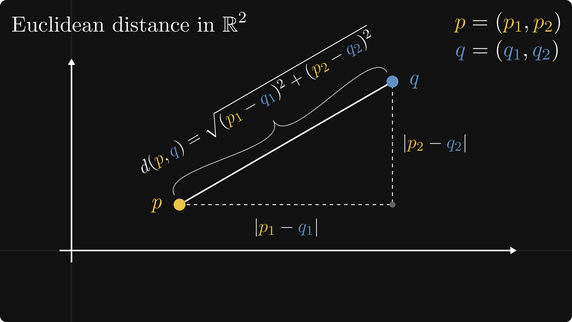
Jumping onto the plane, the Euclidean distance is given by the Pythagorean theorem. Using the two points, we can create a right triangle, with the hypotenuse being the distance line segment between the points.
Here it is for two points P = (p₁, p₂) and Q = (q₁, q₂).
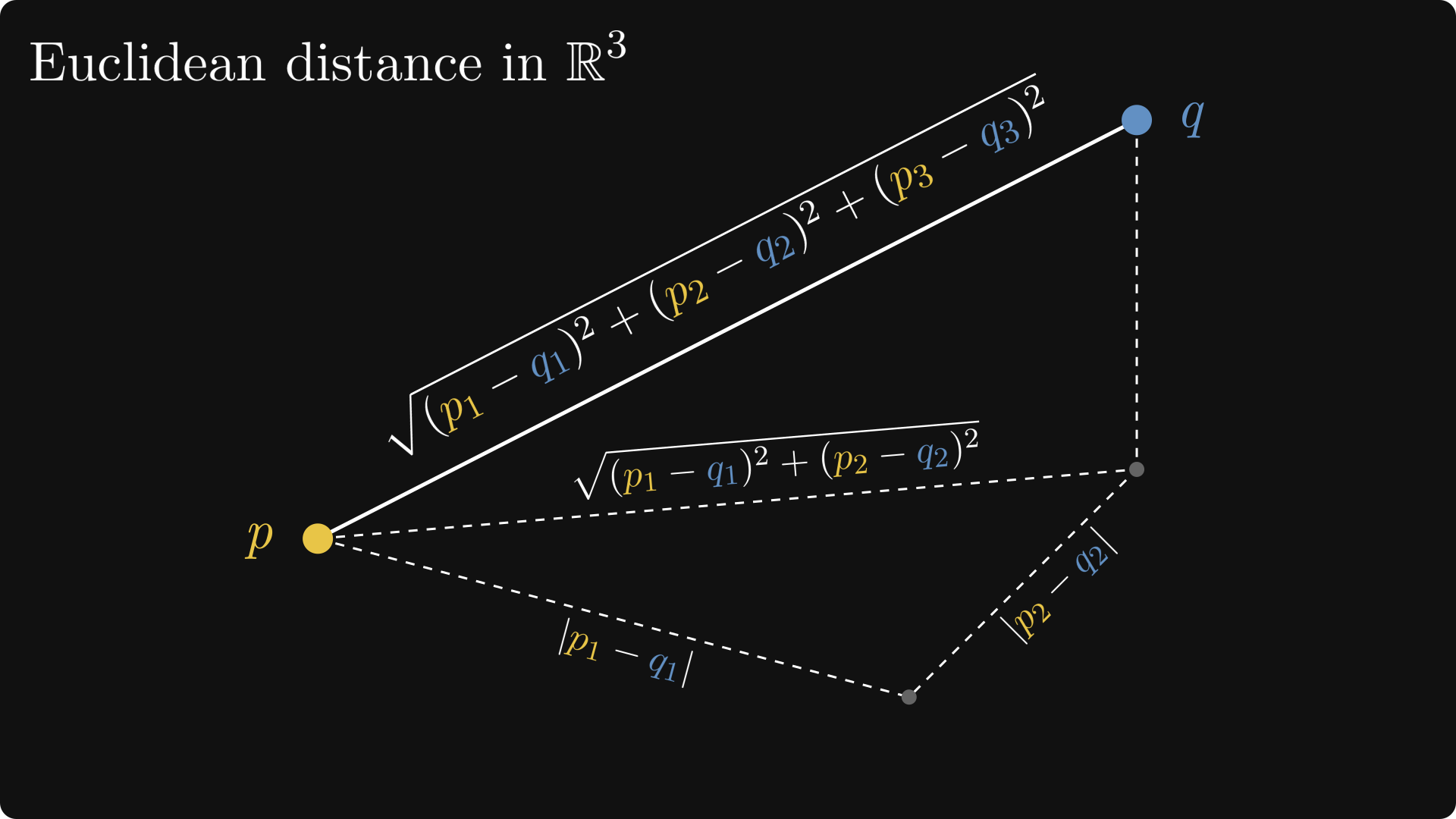
The formula used in the Pythagorean theorem can be extended for the higher dimensions:
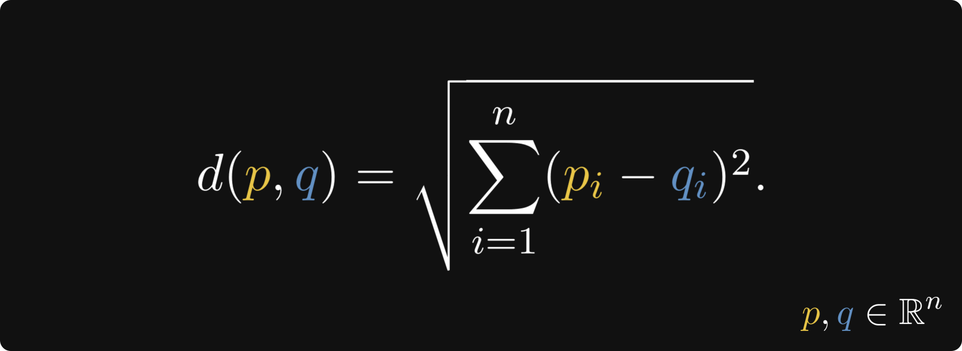
Visualizing more than three dimensions is hard, but in 3D, we can see that this is the repeated application of the Pythagorean theorem.
Manhattan distance
Now, let’s move from the abstract Euclidean space to the streets of Manhattan, New York.
How far is P from Q there? Sure, you can calculate the Euclidean distance between the two points, but it won’t match the distance you have to travel. Why? Because you cannot fly through buildings. You have to get around them!
However, there are multiple ways from P to Q.
Think about this: all possible ways have the same distance! (Given that you don’t go past the destination or back from the start in either direction.)
In mathematics, this distance is called the Manhattan distance, defined by the formula
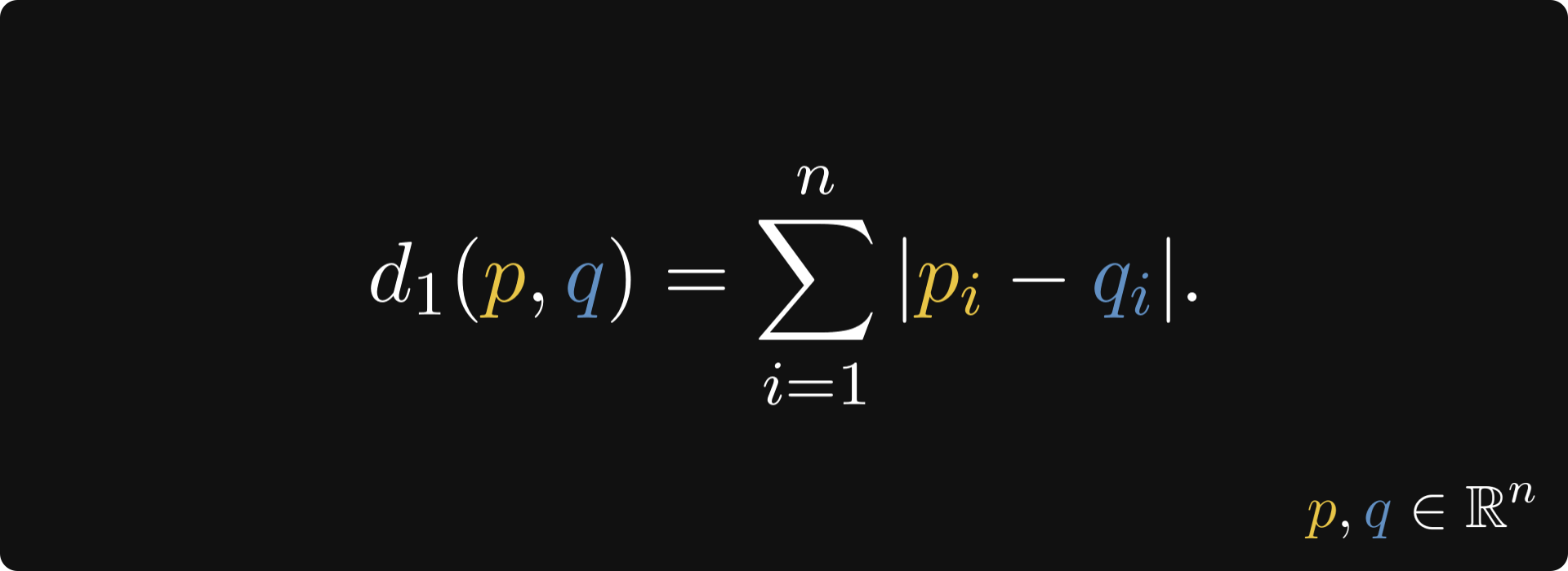
Why should we use this at all? For one, the Manhattan distance is less sensitive to differences in the magnitude of features, which makes it more suitable for dealing with higher dimensional data.
Minkowski distance
If you use kNN through Scikit-learn, you will find the Minkowski distance as the default distance metric.
It’s not an accident: Minkowski is the generalization of both the Euclidean and Manhattan distances.
Here it is in its general form:
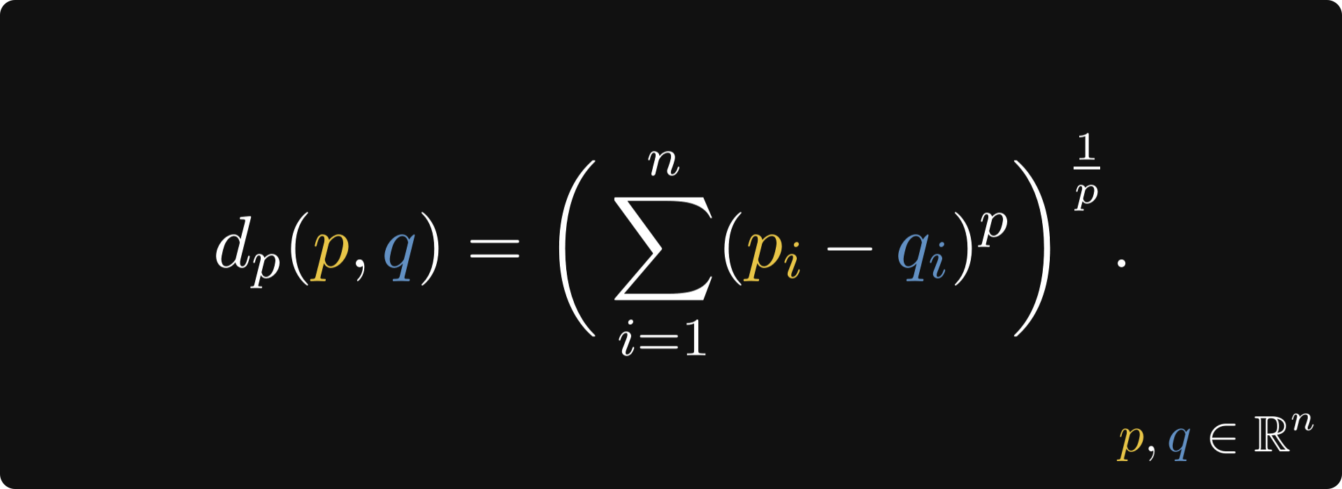
When p = 1, the formula becomes the Manhattan distance, and when p = 2, it becomes the Euclidean distance.
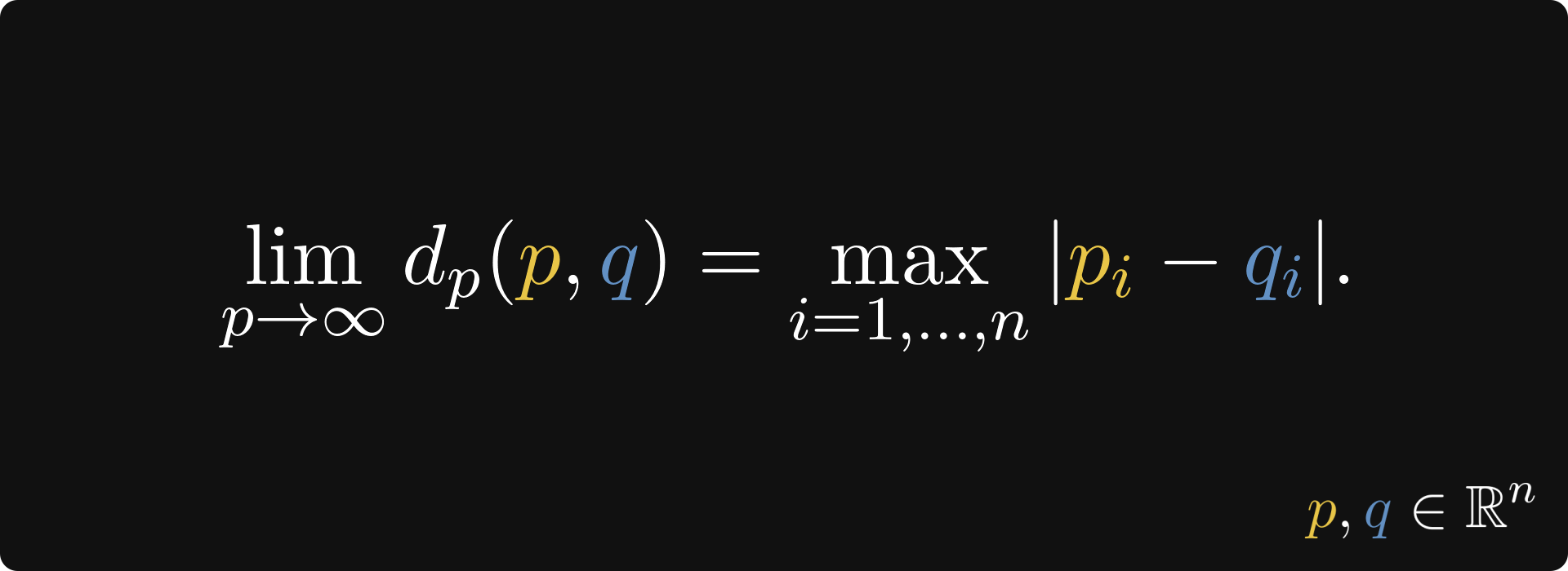
Again, why should we use any other p than 2? As p grows, the Minkowski metric becomes less and less sensitive to individual differences. When p converges to infinity, the metric converges to the largest individual difference between features:
Other ways to use KNN
Let’s turn the table upside down. When we talk about distances, we explore differences. But another way to put it is to talk about similarities. That’s the whole point of classification! We want to find similar points in the space.
For text, image, and other high-dimensional data, we can no longer trust the Eucledian distance.
The curse of dimensionality is a big enemy of kNN. As the number of features grows, the Minkowski metrics hide the subtle differences.
As dimensions increase, variance decreases, so the distance between the pairs will be similar. In high dimensions, the volume of the space is concentrated in the "shell" of the sphere (near the surface). If we chose any two points, they are possibly near the surface and roughly equal distance away from the origin.
One solution to the problem is to apply the cosine similarity as the “distance metric”, defined by
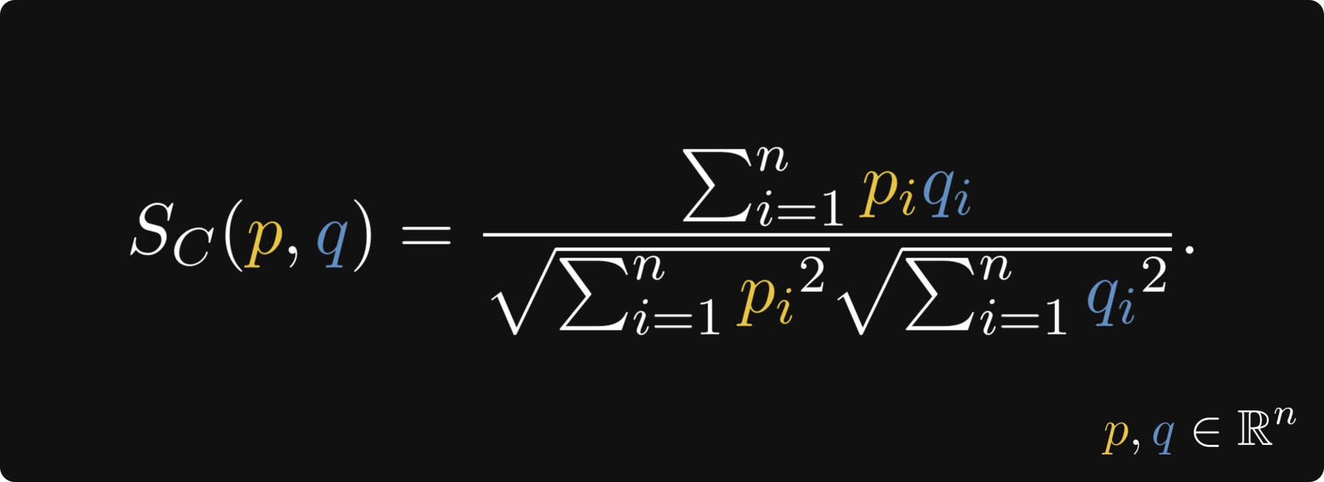
Cosine similarity, focusing only on the direction of the vectors, can sometimes provide better discrimination in such cases. Instead of the distances, we focus on the angles.
Here’s an infographic from Levi that explains what’s up.
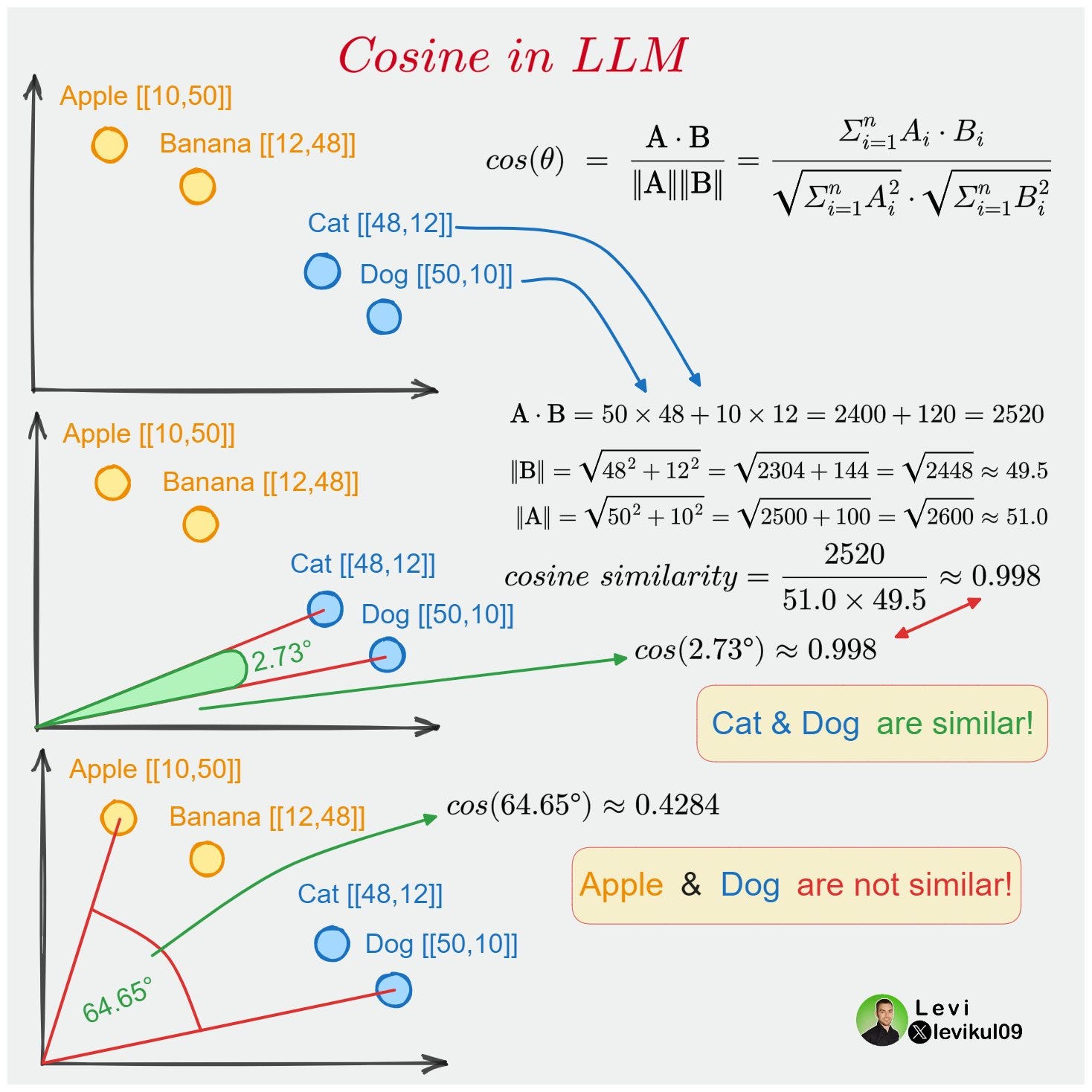
Again, cosine similarity is not limited to the 2D world. The same formula applies to higher dimensions as well!
Lazy vs. Eager Algorithms
Now, it's time to discuss the model's laziness. We can divide ML algorithms into two categories: lazy and eager learners.
Lazy learners don't learn or generalize from the training data. Instead, they store it, and every time a new input comes, they pull it and use it for comparison. The “learning” happens at the time of prediction. kNN is the most prevalent example of lazy learners.
Eager algorithms generalize from the training data by building a model based on the input; this is called the learning phase. In turn, this model is used to make predictions; this is called the prediction phase. For eager algorithms, the training data is irrelevant during the prediction phase; it only looks at the model built by generalizing the training data.
Consider linear regression. In the learning process, the algorithm fits an affine function f(x) = ax + b onto the training data, which is used to make predictions later. The training points are no longer relevant. Neural networks, decision trees, logistic regression, linear regression, or SVM are all eager learners.
Both approaches have their benefits and drawbacks. Since the eager learners generalize from the training data, most computation happens during the training phase. When new data comes, we need to retrain the model. Lazy learners use more power at the prediction phase but are easy to update since no retraining is needed. On the other hand, they need large storage space for huge datasets.
Conclusion
kNN is one of the simplest machine learning algorithms, perhaps the very first we encounter in our journey. (Well, that and linear regression.) Despite its simplicity, it teaches us a ton of valuable lessons.
For one, kNN illuminates the fundamental difference between eager and lazy machine learning, a distinction that is not often considered. Surprisingly, kNN doesn’t learn! It simply memorizes the training data, fetching it upon prediction time.
kNN also shows us the importance of metrics: we must choose them accordingly, considering the nature of our problem. Where the Euclidean metric fails, the cosine similarity might prevail, and vice versa.
Never underestimate the power of kNN; in the right setting, it can even outperform some state-of-the-art transformers!
But that’s a topic for another day.
 | A guest post by
|